Eager execution

Computing gradients

Automatic differentiation is useful for implementing machine learning algorithms such as backpropagation for training neural networks. During eager execution, use tf$GradientTape to trace operations for computing gradients later.

You can use tf$GradientTape to train and/or compute gradients in eager. It is especially useful for complicated training loops.

Since different operations can occur during each call, all forward-pass operations get recorded to a “tape”. To compute the gradient, play the tape backwards and then discard. A particular tf$GradientTape can only compute one gradient; subsequent calls throw a runtime error.

w <- tf$Variable(1)
with(tf$GradientTape() %as% tape, {
  loss <- w * w
})
grad <- tape$gradient(loss, w)
grad

## tf.Tensor(2.0, shape=(), dtype=float32)

Train a model

The following example creates a multi-layer model that classifies the standard MNIST handwritten digits. It demonstrates the optimizer and layer APIs to build trainable graphs in an eager execution environment.

# Fetch and format the mnist data
mnist <- dataset_mnist()
dataset <- tensor_slices_dataset(mnist$train) %>% 
  dataset_map(function(x) {
    x$x <- tf$cast(x$x, tf$float32)/255
    x$x <- tf$expand_dims(x$x, axis = -1L)
    unname(x)
  }) %>% 
  dataset_shuffle(1000) %>% 
  dataset_batch(32)

dataset

## <BatchDataset shapes: ((None, 28, 28, 1), (None,)), types: (tf.float32, tf.int32)>

mnist_model <- keras_model_sequential() %>% 
  layer_conv_2d(filters = 16, kernel_size = c(3,3), activation= "relu",
                input_shape = shape(NULL, NULL, 1)) %>% 
  layer_conv_2d(filters = 16, kernel_size = c(3,3), activation = "relu") %>% 
  layer_global_average_pooling_2d() %>% 
  layer_dense(units = 10)

Even without training, call the model and inspect the output in eager execution:

el <- dataset %>% 
  dataset_take(1) %>% 
  dataset_collect()
mnist_model(el[[1]])

## tf.Tensor(
## [[-8.50985199e-03  9.76161857e-04 -2.50255484e-02 -5.79575971e-02
##   -3.91511843e-02 -2.02112067e-02  1.19331172e-02  2.99258605e-02
##    7.55230756e-03  3.86199094e-02]
##  [-5.54877939e-03  1.90716446e-03 -1.70769673e-02 -3.62131633e-02
##   -2.53974535e-02 -1.38209835e-02  7.40819378e-03  1.79758631e-02
##    5.72366873e-03  2.54252721e-02]
##  [-2.37655244e-03  1.36287510e-03 -1.33525934e-02 -3.33486199e-02
##   -2.12530848e-02 -1.39125455e-02  5.86056244e-03  1.53014306e-02
##    5.15997969e-03  2.24790853e-02]
##  [-8.92254990e-04  2.28004996e-03 -1.07957972e-02 -3.00190244e-02
##   -1.75903179e-02 -1.35528101e-02  4.88691870e-03  1.25359586e-02
##    5.23545966e-03  1.93263516e-02]
##  [-4.21859929e-03  3.05507542e-03 -1.49999214e-02 -3.11945472e-02
##   -2.06255876e-02 -1.27387317e-02  6.34148577e-03  1.41533548e-02
##    5.45461895e-03  2.25168187e-02]
##  [-3.46548553e-03  1.24341354e-03 -1.45013975e-02 -4.30306159e-02
##   -3.16537209e-02 -1.74248051e-02  6.47401158e-03  2.26319134e-02
##    5.64713310e-03  2.93269195e-02]
##  [-6.41194824e-03  1.38130516e-03 -1.84288751e-02 -4.14446481e-02
##   -3.08680199e-02 -1.57348588e-02  7.77957682e-03  2.17617080e-02
##    4.86520818e-03  2.92749219e-02]
##  [-8.39145947e-03 -2.43743139e-04 -2.18558982e-02 -5.35714217e-02
##   -3.83904204e-02 -1.82459299e-02  1.09588886e-02  3.00901663e-02
##    3.97703936e-03  3.47796679e-02]
##  [-6.90627703e-03 -2.02620332e-03 -1.62484460e-02 -4.23779786e-02
##   -3.48815881e-02 -1.46378912e-02  7.04134628e-03  2.60561779e-02
##    2.87065259e-03  3.00167799e-02]
##  [-3.46036465e-03  3.34005570e-03 -1.42491609e-02 -2.86302492e-02
##   -1.86991822e-02 -1.21941017e-02  5.76612214e-03  1.24817807e-02
##    5.39597031e-03  2.08636373e-02]
##  [-6.75824890e-03  1.80363667e-03 -1.81528479e-02 -3.73662151e-02
##   -2.79965084e-02 -1.33580044e-02  7.09015829e-03  1.83111280e-02
##    6.74578175e-03  2.72248089e-02]
##  [-3.44557199e-03  1.44218188e-03 -1.55201033e-02 -3.91926579e-02
##   -3.03197410e-02 -1.78610198e-02  6.71680411e-03  2.06990894e-02
##    5.46659622e-03  2.73653362e-02]
##  [-2.98760762e-03  6.68506909e-05 -1.03480723e-02 -2.65669450e-02
##   -2.34568883e-02 -1.09654916e-02  3.45098414e-03  1.51341530e-02
##    4.49841795e-03  2.06842236e-02]
##  [-6.59199711e-03  1.85408711e-03 -1.94277260e-02 -4.28726152e-02
##   -2.99611464e-02 -1.58806108e-02  9.21235979e-03  2.24604607e-02
##    5.33315912e-03  2.91829202e-02]
##  [-7.55199324e-03 -9.93973459e-04 -2.15730183e-02 -5.56724407e-02
##   -4.60459515e-02 -2.07579192e-02  9.57913976e-03  3.33841294e-02
##    4.62856423e-03  3.92136984e-02]
##  [-2.03214702e-03  4.08457185e-04 -1.21998340e-02 -3.37962173e-02
##   -2.65589673e-02 -1.54427039e-02  4.19362914e-03  1.70531943e-02
##    5.84620563e-03  2.43132822e-02]
##  [-3.81546142e-03  1.21751742e-04 -1.36933727e-02 -3.54161970e-02
##   -2.85060816e-02 -1.41160497e-02  5.15741529e-03  1.88995544e-02
##    5.81339980e-03  2.64615659e-02]
##  [-4.51849913e-03  1.79681068e-04 -1.25195542e-02 -2.85590179e-02
##   -2.36752722e-02 -1.03663774e-02  4.86267731e-03  1.64620187e-02
##    4.00224933e-03  2.16186680e-02]
##  [-6.88880868e-03  2.30632047e-03 -2.50062961e-02 -6.10050745e-02
##   -4.42578457e-02 -2.45542563e-02  1.10575147e-02  3.20139751e-02
##    7.40471063e-03  4.25111316e-02]
##  [-8.04840680e-03 -1.73170422e-03 -2.13432573e-02 -5.59643619e-02
##   -4.14501876e-02 -1.88157260e-02  1.08416816e-02  3.29777822e-02
##    3.58740776e-03  3.77420597e-02]
##  [-2.12463085e-03  1.40806718e-03 -1.62827484e-02 -4.21891250e-02
##   -2.92056706e-02 -1.80202033e-02  6.18648017e-03  1.89643912e-02
##    7.54634384e-03  2.85427365e-02]
##  [-6.24155253e-03  3.68376786e-04 -1.89247429e-02 -4.59269919e-02
##   -3.55105102e-02 -1.77306253e-02  7.98209663e-03  2.48527452e-02
##    5.78143680e-03  3.23706158e-02]
##  [-1.42555241e-03  4.77403111e-04 -1.20030018e-02 -3.56824584e-02
##   -2.53661703e-02 -1.50882667e-02  5.09238290e-03  1.77882873e-02
##    5.66911884e-03  2.43990738e-02]
##  [-1.21319480e-02 -3.38456419e-04 -3.04601416e-02 -6.95648193e-02
##   -5.14865555e-02 -2.32764110e-02  1.34642534e-02  3.88753153e-02
##    5.17100841e-03  4.83683124e-02]
##  [-7.99048692e-03  1.30610866e-03 -2.30237599e-02 -5.47382683e-02
##   -3.83893251e-02 -2.00371165e-02  1.12129143e-02  2.90373228e-02
##    5.98406652e-03  3.79212201e-02]
##  [-6.75235782e-03  9.91679379e-04 -1.80075001e-02 -3.80989239e-02
##   -2.85798106e-02 -1.37160970e-02  7.86706619e-03  2.10245345e-02
##    3.95417260e-03  2.71354374e-02]
##  [-7.98894465e-03  4.55419155e-04 -2.53729578e-02 -6.31851330e-02
##   -4.31225747e-02 -2.33430732e-02  1.32131195e-02  3.43508609e-02
##    5.29513042e-03  4.14416529e-02]
##  [-3.49725038e-03 -2.39763220e-04 -1.08997943e-02 -2.69409642e-02
##   -2.45306063e-02 -1.08287791e-02  3.64527735e-03  1.59635600e-02
##    3.91276646e-03  2.12638490e-02]
##  [-6.46782434e-03 -7.04026374e-04 -1.56770907e-02 -3.86993401e-02
##   -3.16020884e-02 -1.30451052e-02  6.17024768e-03  2.19560675e-02
##    4.18775994e-03  2.79887151e-02]
##  [-5.55107370e-03  2.06118939e-03 -1.58842616e-02 -3.25190350e-02
##   -2.33283471e-02 -1.21178171e-02  6.47215592e-03  1.56531073e-02
##    5.25392406e-03  2.41678189e-02]
##  [-8.96292087e-03 -5.41977119e-04 -2.13856287e-02 -4.84847501e-02
##   -3.47109959e-02 -1.52589623e-02  1.07035376e-02  2.74108090e-02
##    4.38953377e-03  3.33805010e-02]
##  [-5.13768382e-03 -8.29380937e-04 -1.55788297e-02 -4.19435799e-02
##   -3.52306105e-02 -1.68032013e-02  6.36776956e-03  2.41187550e-02
##    5.30361803e-03  3.00990045e-02]], shape=(32, 10), dtype=float32)

While keras models have a builtin training loop (using the fit method), sometimes you need more customization. Here’s an example, of a training loop implemented with eager:

optimizer <- optimizer_adam()
loss_object <- tf$keras$losses$SparseCategoricalCrossentropy(from_logits = TRUE)

loss_history <- list()

Note: Use the assert functions in tf$debugging to check if a condition holds up. This works in eager and graph execution.

train_step <- function(images, labels) {
  with(tf$GradientTape() %as% tape, {
    logits <- mnist_model(images, training = TRUE)
    tf$debugging$assert_equal(logits$shape, shape(32, 10))
    loss_value <- loss_object(labels, logits)
  })
  loss_history <<- append(loss_history, loss_value)
  grads <- tape$gradient(loss_value, mnist_model$trainable_variables)
  optimizer$apply_gradients(
    purrr::transpose(list(grads, mnist_model$trainable_variables))
  )
}

train <- autograph(function() {
  for (epoch in seq_len(3)) {
    for (batch in dataset) {
      train_step(batch[[1]], batch[[2]])
    }
    tf$print("Epoch", epoch, "finished.")
  }
})

train()

history <- loss_history %>% 
  purrr::map(as.numeric) %>% 
  purrr::flatten_dbl()
ggplot2::qplot(x = seq_along(history), y = history, geom = "line")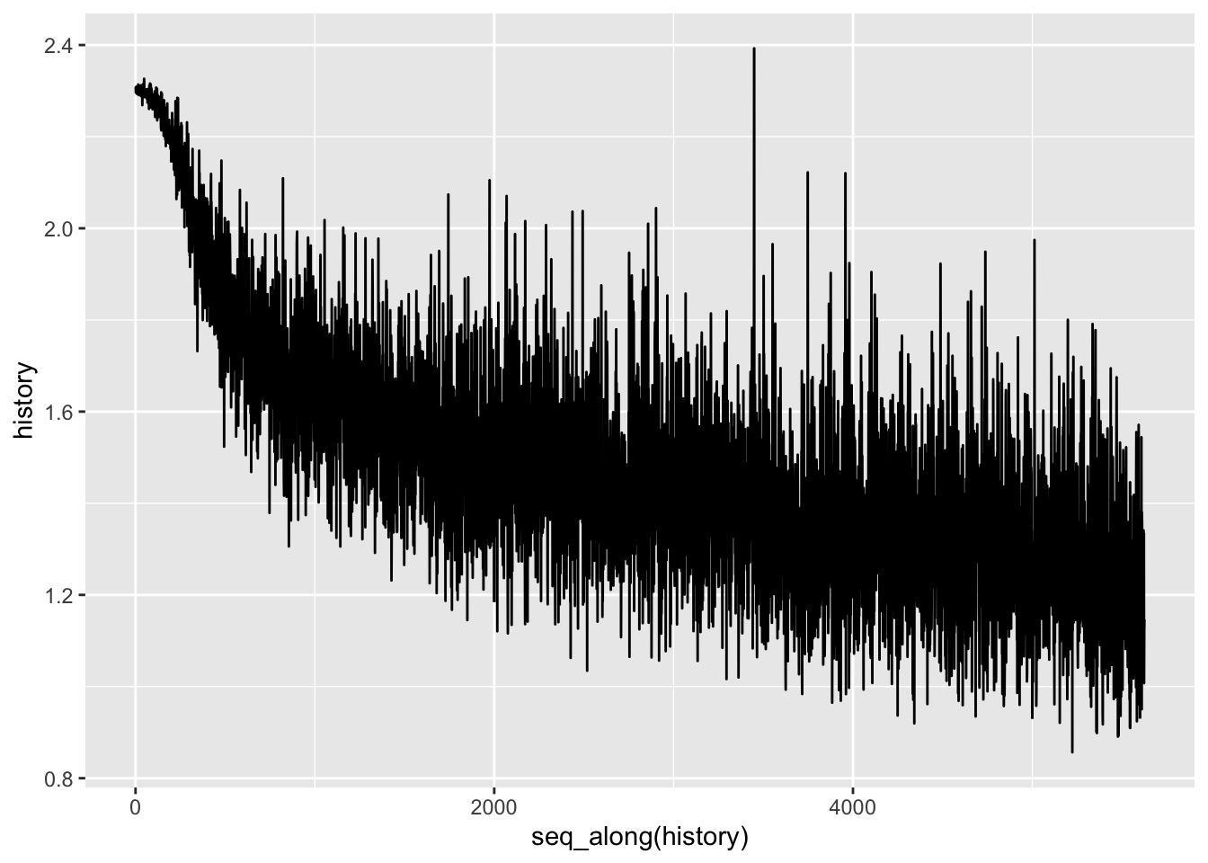

Variables and optimizers

tf$Variable objects store mutable tf$Tensor-like values accessed during training to make automatic differentiation easier.

The collections of variables can be encapsulated into layers or models, along with methods that operate on them. See Custom Keras layers and models for details. The main difference between layers and models is that models add methods like fit, evaluate, and save.

For example, the automatic differentiation example above can be rewritten:

Linear <- function() {
  keras_model_custom(model_fn = function(self) {
    self$w <- tf$Variable(5, name = "weight")
    self$b <- tf$Variable(10, name = "bias")
    function(inputs, mask = NULL, training = TRUE) {
      inputs*self$w + self$b
    }
  }) 
}

# A toy dataset of points around 3 * x + 2
NUM_EXAMPLES <- 2000
training_inputs <- tf$random$normal(shape = shape(NUM_EXAMPLES))
noise <- tf$random$normal(shape = shape(NUM_EXAMPLES))
training_outputs <- training_inputs * 3 + 2 + noise

# The loss function to be optimized
loss <- function(model, inputs, targets) {
  error <- model(inputs) - targets
  tf$reduce_mean(tf$square(error))
}

grad <- function(model, inputs, targets) {
  with(tf$GradientTape() %as% tape, {
    loss_value <- loss(model, inputs, targets)
  })
  tape$gradient(loss_value, list(model$w, model$b))
}

Next:

1. Create the model.
2. The Derivatives of a loss function with respect to model parameters.
3. A strategy for updating the variables based on the derivatives.

model <- Linear()
optimizer <- optimizer_sgd(lr = 0.01)

cat("Initial loss: ", as.numeric(loss(model, training_inputs, training_outputs), "\n"))

## Initial loss:  68.66985

for (i in seq_len(300)) {
  grads <- grad(model, training_inputs, training_outputs)
  optimizer$apply_gradients(purrr::transpose(
    list(grads, list(model$w, model$b))
  ))
  if (i %% 20 == 0)
    cat("Loss at step ", i, ": ", as.numeric(loss(model, training_inputs, training_outputs)), "\n")
}

## Loss at step  20 :  31.23723 
## Loss at step  40 :  14.52059 
## Loss at step  60 :  7.055109 
## Loss at step  80 :  3.721035 
## Loss at step  100 :  2.23201 
## Loss at step  120 :  1.566984 
## Loss at step  140 :  1.269965 
## Loss at step  160 :  1.137304 
## Loss at step  180 :  1.078052 
## Loss at step  200 :  1.051587 
## Loss at step  220 :  1.039765 
## Loss at step  240 :  1.034485 
## Loss at step  260 :  1.032126 
## Loss at step  280 :  1.031073 
## Loss at step  300 :  1.030602

model$w

## <tf.Variable 'weight:0' shape=() dtype=float32, numpy=3.0587368>

model$b

## <tf.Variable 'bias:0' shape=() dtype=float32, numpy=2.0177262>

Note: Variables persist until the last reference to the object is removed, and is the variable is deleted.

Object-based saving

A Keras model includes a convinient save_weights method allowing you to easily create a checkpoint:

save_model_weights_tf(model, "weights")
load_model_weights_tf(model, filepath = "weights")

Using tf$train$Checkpoint you can take full control over this process.

This section is an abbreviated version of the guide to training checkpoints.

x <- tf$Variable(10)
checkpoint <- tf$train$Checkpoint(x = x)

x$assign(2) # Assign a new value to the variables and save.

## <tf.Variable 'UnreadVariable' shape=() dtype=float32, numpy=2.0>

checkpoint_path <- "ckpt/"
checkpoint$save(checkpoint_path)

## [1] "ckpt/-1"

x$assign(11) # Change the variable after saving.

## <tf.Variable 'UnreadVariable' shape=() dtype=float32, numpy=11.0>

checkpoint$restore(tf$train$latest_checkpoint(checkpoint_path))

## <tensorflow.python.training.tracking.util.CheckpointLoadStatus>

x

## <tf.Variable 'Variable:0' shape=() dtype=float32, numpy=2.0>

To save and load models, tf$train$Checkpoint stores the internal state of objects, without requiring hidden variables. To record the state of a model, an optimizer, and a global step, pass them to a tf$train$Checkpoint:

model <- keras_model_sequential() %>% 
  layer_conv_2d(filters = 16, kernel_size = c(3,3), activation = "relu") %>% 
  layer_global_average_pooling_2d() %>% 
  layer_dense(units = 10)

optimizer <- optimizer_adam(lr = 0.001)

checkpoint_dir <- 'path/to/model_dir'
if (!dir.exists(checkpoint_dir))
  dir.create(checkpoint_dir, recursive = TRUE)

checkpoint_prefix <- file.path(checkpoint_dir, "ckpt")

root <- tf$train$Checkpoint(optimizer = optimizer, model = model)

root$save(checkpoint_prefix)

## [1] "path/to/model_dir/ckpt-1"

root$restore(tf$train$latest_checkpoint(checkpoint_dir))

## <tensorflow.python.training.tracking.util.CheckpointLoadStatus>

Note: In many training loops, variables are created after tf\(train\)Checkpoint.restore is called. These variables will be restored as soon as they are created, and assertions are available to ensure that a checkpoint has been fully loaded. See the guide to training checkpoints for details.

Object-oriented metrics

tf$keras$metrics are stored as objects. Update a metric by passing the new data to the callable, and retrieve the result using the tf$keras$metrics$result method, for example:

m <- tf$keras$metrics$Mean("loss")
m(0)

## tf.Tensor(0.0, shape=(), dtype=float32)

m(5)

## tf.Tensor(2.5, shape=(), dtype=float32)

m$result()

## tf.Tensor(2.5, shape=(), dtype=float32)

m(c(8, 9))

## tf.Tensor(5.5, shape=(), dtype=float32)

m$result()

## tf.Tensor(5.5, shape=(), dtype=float32)

Summaries and TensorBoard

TensorBoard is a visualization tool for understanding, debugging and optimizing the model training process. It uses summary events that are written while executing the program.

You can use tf$summary to record summaries of variable in eager execution. For example, to record summaries of loss once every 100 training steps:

logdir <- "./tb/"
writer = tf$summary$create_file_writer(logdir)
tensorboard(log_dir = logdir) # This will open a browser window pointing to Tensorboard

with(writer$as_default(), {
  for (step in seq_len(1000)) {
    # Calculate loss with your real train function.
    loss = 1 - 0.001 * step
    if (step %% 100 == 0)
      tf$summary$scalar('loss', loss, step=step)
  }
})

Dynamic models

tf$GradientTape can also be used in dynamic models. This example for a backtracking line search algorithm looks like normal R code, except there are gradients and is differentiable, despite the complex control flow:

line_search_step <- tf$custom_gradient(autograph(function(fn, init_x, rate = 1) {
  with(tf$GradientTape() %as% tape, {
    tape$watch(init_x)
    value <- fn(init_x)
  })
  grad <- tape$gradient(value, init_x)
  grad_norm <- tf$reduce_sum(grad * grad)
  init_value <- value
  while(value > (init_value - rate * grad_norm)) {
    x <- init_x - rate * grad
    value <- fn(x)
    rate = rate/2
  }
  list(x, value)
}))

Custom gradients

Custom gradients are an easy way to override gradients. Within the forward function, define the gradient with respect to the inputs, outputs, or intermediate results. For example, here’s an easy way to clip the norm of the gradients in the backward pass:

clip_gradient_by_norm <- function(x, norm) {
  y <- tf$identity(x)
  grad_fn <- function(dresult) {
    list(tf$clip_by_norm(dresult, norm), NULL)
  }
  list(y, grad_fn)
}

Custom gradients are commonly used to provide a numerically stable gradient for a sequence of operations:

log1pexp <- function(x) {
  tf$math$log(1 + tf$exp(x))
}

grad_log1pexp <- function(x) {
  with(tf$GradientTape() %as% tape, {
    tape$watch(x)
    value <- log1pexp(x)
  })
  tape$gradient(value, x)
}

# The gradient computation works fine at x = 0.
grad_log1pexp(tf$constant(0))

## tf.Tensor(0.5, shape=(), dtype=float32)

# However, x = 100 fails because of numerical instability.
grad_log1pexp(tf$constant(100))

## tf.Tensor(nan, shape=(), dtype=float32)

Here, the log1pexp function can be analytically simplified with a custom gradient. The implementation below reuses the value for tf$exp(x) that is computed during the forward pass—making it more efficient by eliminating redundant calculations:

log1pexp <- tf$custom_gradient(f = function(x) {
  e <- tf$exp(x)
  grad_fn <- function(dy) {
    dy * (1 - 1/(e + e))
  }
  list(tf$math$log(1 + e), grad_fn)
})

grad_log1pexp <- function(x) {
  with(tf$GradientTape() %as% tape, {
    tape$watch(x)
    value <- log1pexp(x)
  })
  tape$gradient(value, x)
}

# As before, the gradient computation works fine at x = 0.
grad_log1pexp(tf$constant(0))

## tf.Tensor(0.5, shape=(), dtype=float32)

# And the gradient computation also works at x = 100.
grad_log1pexp(tf$constant(100))

## tf.Tensor(1.0, shape=(), dtype=float32)

Benchmarks

For compute-heavy models, such as ResNet50 training on a GPU, eager execution performance is comparable to tf_function execution. But this gap grows larger for models with less computation and there is work to be done for optimizing hot code paths for models with lots of small operations.