Feature Spec interface

Overview

In this document we will demonstrate the basic usage of the feature_spec interface in tfdatasets.

The feature_spec interface is a user friendly interface to feature_columns. It allows us to specify column transformations and representations when working with structured data.

We will use the hearts dataset and it can be loaded with data(hearts).

library(tfdatasets)
library(dplyr)

## 
## Attaching package: 'dplyr'

## The following objects are masked from 'package:stats':
## 
##     filter, lag

## The following objects are masked from 'package:base':
## 
##     intersect, setdiff, setequal, union

data(hearts)

head(hearts)

## # A tibble: 6 x 14
##     age   sex    cp trestbps  chol   fbs restecg thalach exang oldpeak slope
##   <int> <int> <int>    <int> <int> <int>   <int>   <int> <int>   <dbl> <int>
## 1    63     1     1      145   233     1       2     150     0     2.3     3
## 2    67     1     4      160   286     0       2     108     1     1.5     2
## 3    67     1     4      120   229     0       2     129     1     2.6     2
## 4    37     1     3      130   250     0       0     187     0     3.5     3
## 5    41     0     2      130   204     0       2     172     0     1.4     1
## 6    56     1     2      120   236     0       0     178     0     0.8     1
## # … with 3 more variables: ca <int>, thal <chr>, target <int>

We want to train a model to predict the target variable using Keras but, before that we need to prepare the data. We need to transform the categorical variables into some form of dense variable, we usually want to normalize all numeric columns too.

The feature spec interface works with data.frames or TensorFlow datasets objects.

ids_train <- sample.int(nrow(hearts), size = 0.75*nrow(hearts))
hearts_train <- hearts[ids_train,]
hearts_test <- hearts[-ids_train,]

Now let’s start creating our feature specification:

spec <- feature_spec(hearts_train, target ~ .)

The first thing we need to do after creating the feature_spec is decide on the variables’ types.

We can do this by adding steps to the spec object.

spec <- spec %>% 
  step_numeric_column(
    all_numeric(), -cp, -restecg, -exang, -sex, -fbs,
    normalizer_fn = scaler_standard()
  ) %>% 
  step_categorical_column_with_vocabulary_list(thal)

The following steps can be used to define the variable type:

step_numeric_column to define numeric variables
step_categorical_with_vocabulary_list for categorical variables with a fixed vocabulary
step_categorical_column_with_hash_bucket for categorical variables using the hash trick
step_categorical_column_with_identity to store categorical variables as integers
step_categorical_column_with_vocabulary_file when you have the possible vocabulary in a file

When using step_categorical_column_with_vocabulary_list you can also provide a vocabulary argument with the fixed vocabulary. The recipe will find all the unique values in the dataset and use it as the vocabulary.

You can also specify a normalizer_fn to the step_numeric_column. In this case the variable will be transformed by the feature column. Note that the transformation will occur in the TensorFlow Graph, so it must use only TensorFlow ops. Like in the example we offer pre-made normalizers - and they will compute the normalizing function during the recipe preparation.

You can also use selectors like:

starts_with(), ends_with(), matches() etc. (from tidyselect)
all_numeric() to select all numeric variables
all_nominal() to select all strings
has_type("float32") to select based on TensorFlow variable type.

Now we can print the recipe:

spec

## ── Feature Spec ────────────────────────────────────────────────────────────────────────────── 
## A feature_spec with 8 steps.
## Fitted: FALSE 
## ── Steps ───────────────────────────────────────────────────────────────────────────────────── 
## StepCategoricalColumnWithVocabularyList: thal 
## StepNumericColumn: age, trestbps, chol, thalach, oldpeak, slope, ca 
## ── Dense features ──────────────────────────────────────────────────────────────────────────── 
## Feature spec must be fitted before we can detect the dense features.

After specifying the types of the columns you can add transformation steps. For example you may want to bucketize a numeric column:

spec <- spec %>% 
  step_bucketized_column(age, boundaries = c(18, 25, 30, 35, 40, 45, 50, 55, 60, 65))

You can also specify the kind of numeric representation that you want to use for your categorical variables.

spec <- spec %>% 
  step_indicator_column(thal) %>% 
  step_embedding_column(thal, dimension = 2)

Another common transformation is to add interactions between variables using crossed columns.

spec <- spec %>% 
  step_crossed_column(thal_and_age = c(thal, bucketized_age), hash_bucket_size = 1000) %>% 
  step_indicator_column(thal_and_age)

Note that the crossed_column is a categorical column, so we need to also specify what kind of numeric tranformation we want to use. Also note that we can name the transformed variables - each step uses a default naming for columns, eg. bucketized_age is the default name when you use step_bucketized_column with column called age.

With the above code we have created our recipe. Note we can also define the recipe by chaining a sequence of methods:

spec <- feature_spec(hearts_train, target ~ .) %>% 
  step_numeric_column(
    all_numeric(), -cp, -restecg, -exang, -sex, -fbs,
    normalizer_fn = scaler_standard()
  ) %>% 
  step_categorical_column_with_vocabulary_list(thal) %>% 
  step_bucketized_column(age, boundaries = c(18, 25, 30, 35, 40, 45, 50, 55, 60, 65)) %>% 
  step_indicator_column(thal) %>% 
  step_embedding_column(thal, dimension = 2) %>% 
  step_crossed_column(c(thal, bucketized_age), hash_bucket_size = 10) %>%
  step_indicator_column(crossed_thal_bucketized_age)

After defining the recipe we need to fit it. It’s when fitting that we compute the vocabulary list for categorical variables or find the mean and standard deviation for the normalizing functions. Fitting involves evaluating the full dataset, so if you have provided the vocabulary list and your columns are already normalized you can skip the fitting step (TODO).

In our case, we will fit the feature spec, since we didn’t specify the vocabulary list for the categorical variables.

spec_prep <- fit(spec)

After preparing we can see the list of dense features that were defined:

str(spec_prep$dense_features())

## List of 11
##  $ age                                  :NumericColumn(key='age', shape=(1,), default_value=None, dtype=tf.float32, normalizer_fn=<function make_python_function.<locals>.python_function at 0x1335af6a8>)
##  $ trestbps                             :NumericColumn(key='trestbps', shape=(1,), default_value=None, dtype=tf.float32, normalizer_fn=<function make_python_function.<locals>.python_function at 0x1335af7b8>)
##  $ chol                                 :NumericColumn(key='chol', shape=(1,), default_value=None, dtype=tf.float32, normalizer_fn=<function make_python_function.<locals>.python_function at 0x1335af8c8>)
##  $ thalach                              :NumericColumn(key='thalach', shape=(1,), default_value=None, dtype=tf.float32, normalizer_fn=<function make_python_function.<locals>.python_function at 0x1335afea0>)
##  $ oldpeak                              :NumericColumn(key='oldpeak', shape=(1,), default_value=None, dtype=tf.float32, normalizer_fn=<function make_python_function.<locals>.python_function at 0x1335aff28>)
##  $ slope                                :NumericColumn(key='slope', shape=(1,), default_value=None, dtype=tf.float32, normalizer_fn=<function make_python_function.<locals>.python_function at 0x1335af158>)
##  $ ca                                   :NumericColumn(key='ca', shape=(1,), default_value=None, dtype=tf.float32, normalizer_fn=<function make_python_function.<locals>.python_function at 0x1335af598>)
##  $ bucketized_age                       :BucketizedColumn(source_column=NumericColumn(key='age', shape=(1,), default_value=None, dtype=tf.float32, normalizer_fn=<function make_python_function.<locals>.python_function at 0x1335af6a8>), boundaries=(18.0, 25.0, 30.0, 35.0, 40.0, 45.0, 50.0, 55.0, 60.0, 65.0))
##  $ indicator_thal                       :IndicatorColumn(categorical_column=VocabularyListCategoricalColumn(key='thal', vocabulary_list=('1', '2', 'fixed', 'normal', 'reversible'), dtype=tf.string, default_value=-1, num_oov_buckets=0))
##  $ embedding_thal                       :EmbeddingColumn(categorical_column=VocabularyListCategoricalColumn(key='thal', vocabulary_list=('1', '2', 'fixed', 'normal', 'reversible'), dtype=tf.string, default_value=-1, num_oov_buckets=0), dimension=2, combiner='mean', initializer=<tensorflow.python.ops.init_ops.TruncatedNormal>, ckpt_to_load_from=None, tensor_name_in_ckpt=None, max_norm=None, trainable=True)
##  $ indicator_crossed_thal_bucketized_age:IndicatorColumn(categorical_column=CrossedColumn(keys=(VocabularyListCategoricalColumn(key='thal', vocabulary_list=('1', '2', 'fixed', 'normal', 'reversible'), dtype=tf.string, default_value=-1, num_oov_buckets=0), BucketizedColumn(source_column=NumericColumn(key='age', shape=(1,), default_value=None, dtype=tf.float32, normalizer_fn=<function make_python_function.<locals>.python_function at 0x1335af6a8>), boundaries=(18.0, 25.0, 30.0, 35.0, 40.0, 45.0, 50.0, 55.0, 60.0, 65.0))), hash_bucket_size=10.0, hash_key=None))

Now we are ready to define our model in Keras. We will use a specialized layer_dense_features that knows what to do with the feature columns specification.

We also use a new layer_input_from_dataset that is useful to create a Keras input object copying the structure from a data.frame or TensorFlow dataset.

library(keras)

input <- layer_input_from_dataset(hearts_train %>% select(-target))

output <- input %>% 
  layer_dense_features(dense_features(spec_prep)) %>% 
  layer_dense(units = 32, activation = "relu") %>% 
  layer_dense(units = 1, activation = "sigmoid")

model <- keras_model(input, output)

model %>% compile(
  loss = loss_binary_crossentropy, 
  optimizer = "adam", 
  metrics = "binary_accuracy"
)

We can finally train the model on the dataset:

history <- model %>% 
  fit(
    x = hearts_train %>% select(-target),
    y = hearts_train$target, 
    epochs = 15, 
    validation_split = 0.2
  )

## Train on 181 samples, validate on 46 samples
## Epoch 1/15
## 
 32/181 [====>.........................] - ETA: 3s - loss: 0.5888 - binary_accuracy: 0.7188
181/181 [==============================] - 1s 6ms/sample - loss: 0.5800 - binary_accuracy: 0.7569 - val_loss: 0.5503 - val_binary_accuracy: 0.8043
## Epoch 2/15
## 
 32/181 [====>.........................] - ETA: 0s - loss: 0.5467 - binary_accuracy: 0.7812
181/181 [==============================] - 0s 195us/sample - loss: 0.5454 - binary_accuracy: 0.7790 - val_loss: 0.5166 - val_binary_accuracy: 0.8478
## Epoch 3/15
## 
 32/181 [====>.........................] - ETA: 0s - loss: 0.5495 - binary_accuracy: 0.7500
181/181 [==============================] - 0s 141us/sample - loss: 0.5141 - binary_accuracy: 0.8122 - val_loss: 0.4894 - val_binary_accuracy: 0.8478
## Epoch 4/15
## 
 32/181 [====>.........................] - ETA: 0s - loss: 0.4654 - binary_accuracy: 0.9062
181/181 [==============================] - 0s 154us/sample - loss: 0.4892 - binary_accuracy: 0.8232 - val_loss: 0.4668 - val_binary_accuracy: 0.8478
## Epoch 5/15
## 
 32/181 [====>.........................] - ETA: 0s - loss: 0.5353 - binary_accuracy: 0.8750
181/181 [==============================] - 0s 142us/sample - loss: 0.4673 - binary_accuracy: 0.8287 - val_loss: 0.4496 - val_binary_accuracy: 0.8478
## Epoch 6/15
## 
 32/181 [====>.........................] - ETA: 0s - loss: 0.4931 - binary_accuracy: 0.8125
181/181 [==============================] - 0s 142us/sample - loss: 0.4507 - binary_accuracy: 0.8177 - val_loss: 0.4347 - val_binary_accuracy: 0.8478
## Epoch 7/15
## 
 32/181 [====>.........................] - ETA: 0s - loss: 0.5265 - binary_accuracy: 0.7812
181/181 [==============================] - 0s 151us/sample - loss: 0.4352 - binary_accuracy: 0.8232 - val_loss: 0.4237 - val_binary_accuracy: 0.8478
## Epoch 8/15
## 
 32/181 [====>.........................] - ETA: 0s - loss: 0.3913 - binary_accuracy: 0.8750
181/181 [==============================] - 0s 150us/sample - loss: 0.4237 - binary_accuracy: 0.8177 - val_loss: 0.4146 - val_binary_accuracy: 0.8696
## Epoch 9/15
## 
 32/181 [====>.........................] - ETA: 0s - loss: 0.3618 - binary_accuracy: 0.9375
181/181 [==============================] - 0s 150us/sample - loss: 0.4130 - binary_accuracy: 0.8232 - val_loss: 0.4079 - val_binary_accuracy: 0.8696
## Epoch 10/15
## 
 32/181 [====>.........................] - ETA: 0s - loss: 0.4295 - binary_accuracy: 0.7812
181/181 [==============================] - 0s 146us/sample - loss: 0.4033 - binary_accuracy: 0.8232 - val_loss: 0.4034 - val_binary_accuracy: 0.8696
## Epoch 11/15
## 
 32/181 [====>.........................] - ETA: 0s - loss: 0.3490 - binary_accuracy: 0.8750
181/181 [==============================] - 0s 144us/sample - loss: 0.3953 - binary_accuracy: 0.8232 - val_loss: 0.4001 - val_binary_accuracy: 0.8696
## Epoch 12/15
## 
 32/181 [====>.........................] - ETA: 0s - loss: 0.4143 - binary_accuracy: 0.7500
181/181 [==============================] - 0s 145us/sample - loss: 0.3879 - binary_accuracy: 0.8122 - val_loss: 0.3971 - val_binary_accuracy: 0.8696
## Epoch 13/15
## 
 32/181 [====>.........................] - ETA: 0s - loss: 0.2370 - binary_accuracy: 0.9688
181/181 [==============================] - 0s 150us/sample - loss: 0.3820 - binary_accuracy: 0.8177 - val_loss: 0.3950 - val_binary_accuracy: 0.8696
## Epoch 14/15
## 
 32/181 [====>.........................] - ETA: 0s - loss: 0.4100 - binary_accuracy: 0.7812
181/181 [==============================] - 0s 154us/sample - loss: 0.3762 - binary_accuracy: 0.8232 - val_loss: 0.3939 - val_binary_accuracy: 0.8696
## Epoch 15/15
## 
 32/181 [====>.........................] - ETA: 0s - loss: 0.3385 - binary_accuracy: 0.8750
181/181 [==============================] - 0s 142us/sample - loss: 0.3710 - binary_accuracy: 0.8177 - val_loss: 0.3934 - val_binary_accuracy: 0.8696

plot(history)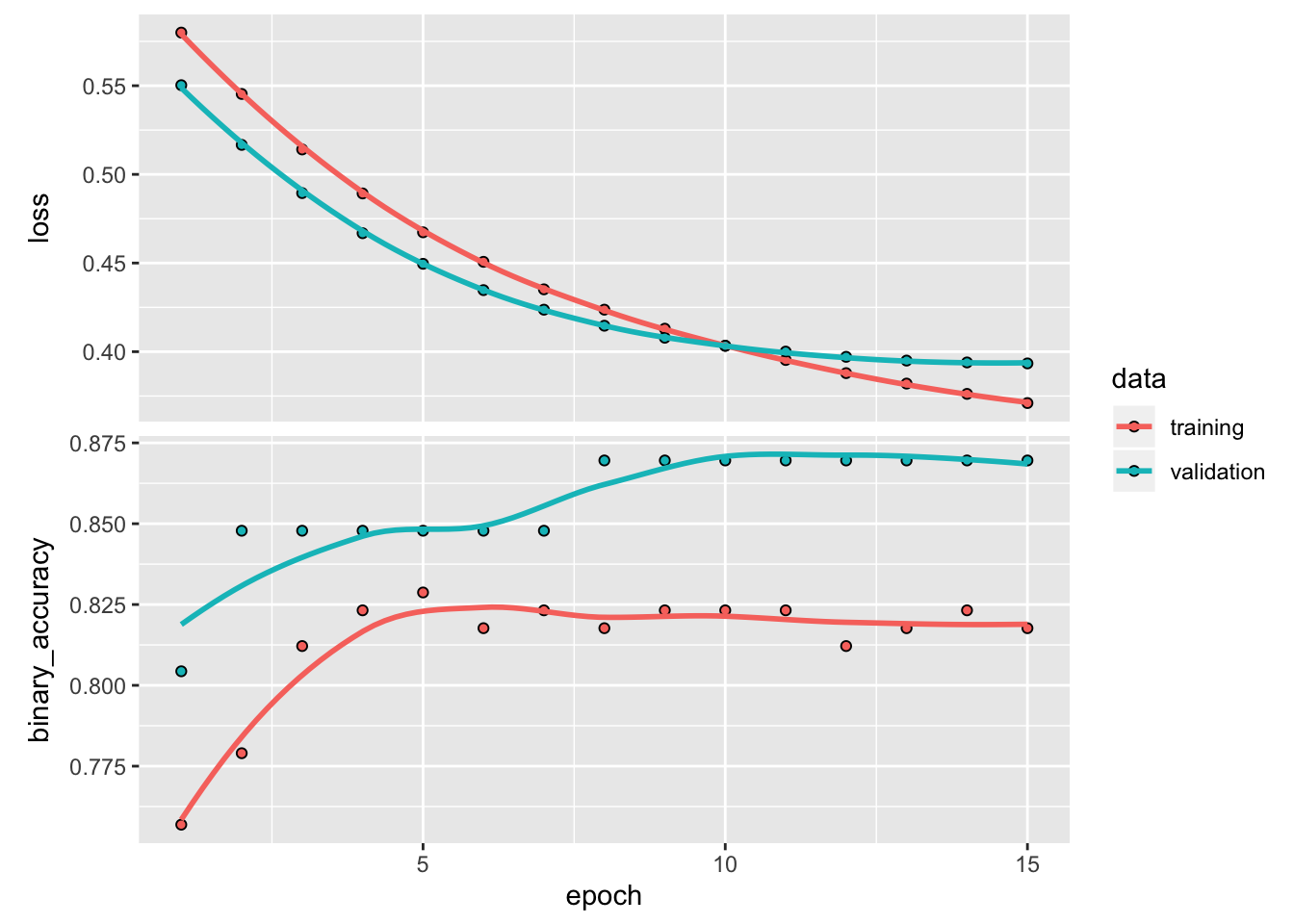

Finally we can make predictions in the test set and calculate performance metrics like the AUC of the ROC curve:

hearts_test$pred <- predict(model, hearts_test)
Metrics::auc(hearts_test$target, hearts_test$pred)

## [1] 0.9232303