TensorFlow Hub with Keras
TensorFlow Hub is a way to share pretrained model components. See the TensorFlow Module Hub for a searchable listing of pre-trained models. This tutorial demonstrates:
- How to use TensorFlow Hub with Keras.
- How to do image classification using TensorFlow Hub.
- How to do simple transfer learning.
Setup
An ImageNet classifier
Download the classifier
Use layer_hub to load a mobilenet and transform it into a Keras layer.
Any TensorFlow 2 compatible image classifier URL from tfhub.dev will work here.
classifier_url <- "https://tfhub.dev/google/tf2-preview/mobilenet_v2/classification/2"
mobilenet_layer <- layer_hub(handle = classifier_url)
#>
#> Done!
We can then create our Keras model:
input <- layer_input(shape = c(224, 224, 3))
output <- input %>%
  mobilenet_layer()

model <- keras_model(input, output)
Run it on a single image
Download a single image to try the model on.
img <- image_read('https://storage.googleapis.com/download.tensorflow.org/example_images/grace_hopper.jpg') %>%
  image_resize(geometry = "224x224x3!") %>%
  image_data() %>%
  as.numeric() %>%
  abind::abind(along = 0) # expand to batch dimension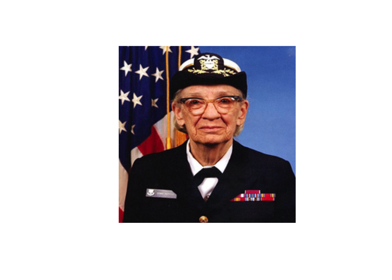
result <- predict(model, img)
mobilenet_decode_predictions(result[,-1, drop = FALSE])
#> [[1]]
#>   class_name class_description    score
#> 1  n03763968  military_uniform 9.355025
#> 2  n03787032       mortarboard 5.400680
#> 3  n02817516          bearskin 5.297816
#> 4  n04350905              suit 5.200010
#> 5  n09835506        ballplayer 4.792098
Simple transfer learning
Using TF Hub it is simple to retrain the top layer of the model to recognize the classes in our dataset.
Dataset
For this example you will use the TensorFlow flowers dataset:
data_root <- pins::pin("https://storage.googleapis.com/download.tensorflow.org/example_images/flower_photos.tgz", "flower_photos")
data_root <- fs::path_dir(fs::path_dir(data_root[100])) # go down 2 levels
The simplest way to load this data into our model is using image_data_generator
All of TensorFlow Hub’s image modules expect float inputs in the [0, 1] range. Use the image_data_generator’s rescale parameter to achieve this.
image_generator <- image_data_generator(rescale = 1/255, validation_split = 0.2)
training_data <- flow_images_from_directory(
  directory = data_root,
  generator = image_generator,
  target_size = c(224, 224),
  subset = "training"
)
#> Found 2939 images belonging to 5 classes.

validation_data <- flow_images_from_directory(
  directory = data_root,
  generator = image_generator,
  target_size = c(224, 224),
  subset = "validation"
)
#> Found 731 images belonging to 5 classes.
The resulting object is an iterator that returns image_batch, label_batch pairs.
Download the headless model
TensorFlow Hub also distributes models without the top classification layer. These can be used to easily do transfer learning.
Any Tensorflow 2 compatible image feature vector URL from tfhub.dev will work here.
feature_extractor_url <- "https://tfhub.dev/google/tf2-preview/mobilenet_v2/feature_vector/2"
feature_extractor_layer <- layer_hub(handle = feature_extractor_url)
Attach a classification head
Now we can create our classification model by attaching a classification head into the feature extractor layer. We define the following model:
input <- layer_input(shape = c(224, 224, 3))
output <- input %>%
  feature_extractor_layer() %>%
  layer_dense(units = training_data$num_classes, activation = "softmax")

model <- keras_model(input, output)
summary(model)
#> Model: "model_1"
#> ________________________________________________________________________________
#> Layer (type)                        Output Shape                    Param #
#> ================================================================================
#> input_2 (InputLayer)                [(None, 224, 224, 3)]           0
#> ________________________________________________________________________________
#> keras_layer_1 (KerasLayer)          (None, 1280)                    2257984
#> ________________________________________________________________________________
#> dense (Dense)                       (None, 5)                       6405
#> ================================================================================
#> Total params: 2,264,389
#> Trainable params: 6,405
#> Non-trainable params: 2,257,984
#> ________________________________________________________________________________
Train the model
We can now train our model in the same way we would train any other Keras model.
We first use compile to configure the training process:
model %>%
  compile(
    loss = "categorical_crossentropy",
    optimizer = "adam",
    metrics = "acc"
  )
We can then use the fit function to fit our model.
model %>%
  fit_generator(
    training_data,
    steps_per_epoch = training_data$n/training_data$batch_size,
    validation_data = validation_data
  )
#>
 1/91 [..............................] - ETA: 7:07 - loss: 1.8092 - acc: 0.2188
 2/91 [..............................] - ETA: 5:08 - loss: 1.8743 - acc: 0.1719
 3/91 [..............................] - ETA: 4:55 - loss: 1.8324 - acc: 0.1771
 4/91 [>.............................] - ETA: 4:29 - loss: 1.7727 - acc: 0.2188
 5/91 [>.............................] - ETA: 4:17 - loss: 1.7390 - acc: 0.2375
 6/91 [>.............................] - ETA: 4:02 - loss: 1.6711 - acc: 0.2812
 7/91 [=>............................] - ETA: 3:52 - loss: 1.6428 - acc: 0.2946
 8/91 [=>............................] - ETA: 3:42 - loss: 1.6052 - acc: 0.3242
 9/91 [=>............................] - ETA: 3:33 - loss: 1.5795 - acc: 0.3333
10/91 [==>...........................] - ETA: 3:27 - loss: 1.5399 - acc: 0.3438
11/91 [==>...........................] - ETA: 3:22 - loss: 1.5016 - acc: 0.3665
12/91 [==>...........................] - ETA: 3:18 - loss: 1.4670 - acc: 0.3854
13/91 [===>..........................] - ETA: 3:15 - loss: 1.4373 - acc: 0.4062
14/91 [===>..........................] - ETA: 3:14 - loss: 1.3955 - acc: 0.4286
15/91 [===>..........................] - ETA: 3:12 - loss: 1.3622 - acc: 0.4479
16/91 [====>.........................] - ETA: 3:09 - loss: 1.3322 - acc: 0.4590
17/91 [====>.........................] - ETA: 3:06 - loss: 1.3177 - acc: 0.4651
18/91 [====>.........................] - ETA: 3:03 - loss: 1.2965 - acc: 0.4774
19/91 [=====>........................] - ETA: 2:59 - loss: 1.2761 - acc: 0.4901
20/91 [=====>........................] - ETA: 2:55 - loss: 1.2566 - acc: 0.4969
21/91 [=====>........................] - ETA: 2:51 - loss: 1.2477 - acc: 0.5000
22/91 [======>.......................] - ETA: 2:48 - loss: 1.2270 - acc: 0.5071
23/91 [======>.......................] - ETA: 2:46 - loss: 1.2074 - acc: 0.5149
24/91 [======>.......................] - ETA: 2:45 - loss: 1.1892 - acc: 0.5234
25/91 [=======>......................] - ETA: 2:42 - loss: 1.1740 - acc: 0.5300
26/91 [=======>......................] - ETA: 2:40 - loss: 1.1698 - acc: 0.5288
27/91 [=======>......................] - ETA: 2:38 - loss: 1.1517 - acc: 0.5370
28/91 [========>.....................] - ETA: 2:36 - loss: 1.1376 - acc: 0.5435
29/91 [========>.....................] - ETA: 2:33 - loss: 1.1258 - acc: 0.5506
30/91 [========>.....................] - ETA: 2:31 - loss: 1.1093 - acc: 0.5604
31/91 [=========>....................] - ETA: 2:28 - loss: 1.0957 - acc: 0.5655
32/91 [=========>....................] - ETA: 2:25 - loss: 1.0895 - acc: 0.5703
33/91 [=========>....................] - ETA: 2:22 - loss: 1.0769 - acc: 0.5758
34/91 [==========>...................] - ETA: 2:20 - loss: 1.0666 - acc: 0.5809
35/91 [==========>...................] - ETA: 2:17 - loss: 1.0581 - acc: 0.5848
36/91 [==========>...................] - ETA: 2:14 - loss: 1.0487 - acc: 0.5885
37/91 [===========>..................] - ETA: 2:14 - loss: 1.0448 - acc: 0.5912
38/91 [===========>..................] - ETA: 2:11 - loss: 1.0406 - acc: 0.5904
39/91 [===========>..................] - ETA: 2:08 - loss: 1.0314 - acc: 0.5945
40/91 [============>.................] - ETA: 2:05 - loss: 1.0197 - acc: 0.5992
41/91 [============>.................] - ETA: 2:02 - loss: 1.0089 - acc: 0.6037
42/91 [============>.................] - ETA: 2:00 - loss: 0.9983 - acc: 0.6102
43/91 [=============>................] - ETA: 1:57 - loss: 0.9919 - acc: 0.6142
44/91 [=============>................] - ETA: 1:54 - loss: 0.9812 - acc: 0.6187
45/91 [=============>................] - ETA: 1:52 - loss: 0.9686 - acc: 0.6265
46/91 [==============>...............] - ETA: 1:50 - loss: 0.9608 - acc: 0.6299
47/91 [==============>...............] - ETA: 1:47 - loss: 0.9559 - acc: 0.6324
48/91 [==============>...............] - ETA: 1:44 - loss: 0.9480 - acc: 0.6349
49/91 [===============>..............] - ETA: 1:41 - loss: 0.9416 - acc: 0.6379
50/91 [===============>..............] - ETA: 1:39 - loss: 0.9355 - acc: 0.6414
51/91 [===============>..............] - ETA: 1:36 - loss: 0.9256 - acc: 0.6460
52/91 [================>.............] - ETA: 1:33 - loss: 0.9165 - acc: 0.6498
53/91 [================>.............] - ETA: 1:31 - loss: 0.9116 - acc: 0.6517
54/91 [================>.............] - ETA: 1:28 - loss: 0.9029 - acc: 0.6547
55/91 [=================>............] - ETA: 1:26 - loss: 0.8985 - acc: 0.6564
56/91 [=================>............] - ETA: 1:23 - loss: 0.8906 - acc: 0.6603
57/91 [=================>............] - ETA: 1:21 - loss: 0.8815 - acc: 0.6647
58/91 [==================>...........] - ETA: 1:18 - loss: 0.8734 - acc: 0.6694
59/91 [==================>...........] - ETA: 1:16 - loss: 0.8679 - acc: 0.6718
60/91 [==================>...........] - ETA: 1:14 - loss: 0.8637 - acc: 0.6736
61/91 [===================>..........] - ETA: 1:11 - loss: 0.8552 - acc: 0.6780
62/91 [===================>..........] - ETA: 1:09 - loss: 0.8562 - acc: 0.6766
63/91 [===================>..........] - ETA: 1:06 - loss: 0.8476 - acc: 0.6803
64/91 [====================>.........] - ETA: 1:04 - loss: 0.8447 - acc: 0.6814
65/91 [====================>.........] - ETA: 1:02 - loss: 0.8403 - acc: 0.6824
66/91 [====================>.........] - ETA: 59s - loss: 0.8321 - acc: 0.6858
67/91 [=====================>........] - ETA: 57s - loss: 0.8249 - acc: 0.6891
68/91 [=====================>........] - ETA: 55s - loss: 0.8221 - acc: 0.6909
69/91 [=====================>........] - ETA: 53s - loss: 0.8202 - acc: 0.6913
70/91 [======================>.......] - ETA: 50s - loss: 0.8141 - acc: 0.6944
71/91 [======================>.......] - ETA: 48s - loss: 0.8113 - acc: 0.6952
72/91 [======================>.......] - ETA: 46s - loss: 0.8052 - acc: 0.6981
73/91 [=======================>......] - ETA: 44s - loss: 0.8003 - acc: 0.7006
74/91 [=======================>......] - ETA: 41s - loss: 0.7977 - acc: 0.7025
75/91 [=======================>......] - ETA: 39s - loss: 0.7908 - acc: 0.7052
76/91 [========================>.....] - ETA: 37s - loss: 0.7844 - acc: 0.7087
77/91 [========================>.....] - ETA: 34s - loss: 0.7796 - acc: 0.7109
78/91 [========================>.....] - ETA: 32s - loss: 0.7757 - acc: 0.7122
79/91 [=========================>....] - ETA: 29s - loss: 0.7704 - acc: 0.7142
80/91 [=========================>....] - ETA: 27s - loss: 0.7683 - acc: 0.7143
81/91 [=========================>....] - ETA: 25s - loss: 0.7649 - acc: 0.7151
82/91 [==========================>...] - ETA: 22s - loss: 0.7597 - acc: 0.7171
83/91 [==========================>...] - ETA: 20s - loss: 0.7551 - acc: 0.7194
84/91 [==========================>...] - ETA: 17s - loss: 0.7523 - acc: 0.7201
85/91 [===========================>..] - ETA: 15s - loss: 0.7490 - acc: 0.7215
86/91 [===========================>..] - ETA: 12s - loss: 0.7444 - acc: 0.7233
87/91 [===========================>..] - ETA: 9s - loss: 0.7397 - acc: 0.7258
88/91 [============================>.] - ETA: 7s - loss: 0.7385 - acc: 0.7264
89/91 [============================>.] - ETA: 4s - loss: 0.7350 - acc: 0.7278
90/91 [============================>.] - ETA: 2s - loss: 0.7313 - acc: 0.7290
91/91 [==============================] - 239s 3s/step - loss: 0.7272 - acc: 0.7303 - val_loss: 0.4682 - val_acc: 0.8372
You can then export your model with:
save_model_tf(model, "model")You can also reload the model_from_saved_model function. Note that you need to
pass the custom_object with the definition of the KerasLayer since it/s not
a default Keras layer.
reloaded_model <- load_model_tf("model")We can verify that the predictions of both the trained model and the reloaded model are equal:
steps <- as.integer(validation_data$n/validation_data$batch_size)
all.equal(
  predict_generator(model, validation_data, steps = steps),
  predict_generator(reloaded_model, validation_data, steps = steps),
)
#> [1] TRUE
The saved model can also be loaded for inference later or be converted to TFLite or TFjs.