Custom training: basics
In the previous tutorial, you covered the TensorFlow APIs for automatic differentiation—a basic building block for machine learning. In this tutorial, you will use the TensorFlow primitives introduced in the prior tutorials to do some simple machine learning.
TensorFlow also includes Keras —a high-level neural network API that provides useful abstractions to reduce boilerplate and makes TensorFlow easier to use without sacrificing flexibility and performance. We strongly recommend the Keras API for development. However, in this short tutorial you will learn how to train a neural network from first principles to establish a strong foundation.
Variables
Tensors in TensorFlow are immutable stateless objects. Machine learning models, however, must have changing state: as your model trains, the same code to compute predictions should behave differently over time (hopefully with a lower loss!).
TensorFlow has stateful operations built-in, and these are often easier than using low-level R representations for your state. Use tf$Variable to represent weights in a model.
A tf$Variable object stores a value and implicitly reads from this stored value. There are operations (tf.assign_sub, tf.scatter_update, etc.) that manipulate the value stored in a TensorFlow variable.
v <- tf$Variable(1)

# Use Python's `assert` as a debugging statement to test the condition
as.numeric(v) == 1
## [1] TRUE## <tf.Variable 'UnreadVariable' shape=() dtype=float32, numpy=3.0>## [1] TRUE## <tf.Variable 'UnreadVariable' shape=() dtype=float32, numpy=9.0>## [1] TRUEComputations using tf$Variable are automatically traced when computing gradients. For variables that represent embeddings, TensorFlow will do sparse updates by default, which are more computation and memory efficient.
A tf$Variable is also a way to show a reader of your code that a piece of state is mutable.
Fit a linear model
Let’s use the concepts you have learned so far—Tensor, Variable, and GradientTape—to build and train a simple model. This typically involves a few steps:
- Define the model.
- Define a loss function.
- Obtain training data.
- Run through the training data and use an “optimizer” to adjust the variables to fit the data.
Here, you’ll create a simple linear model, f(x) = x * W + b, which has two variables: W (weights) and b (bias). You’ll synthesize data such that a well trained model would have W = 3.0 and b = 2.0.
Define the model
You may organize your TensorFlow code to build models the way you prefer, here we will suggest using an R6 class.
Model <- R6::R6Class(
  classname = "Model",
  public = list(
    W = NULL,
    b = NULL,

    initialize = function() {
      self$W <- tf$Variable(5)
      self$b <- tf$Variable(0)
    },

    call = function(x) {
      self$W*x + self$b
    }

  )
)

model <- Model$new()
model$call(3)
## tf.Tensor(15.0, shape=(), dtype=float32)Define the loss function
A loss function measures how well the output of a model for a given input matches the target output. The goal is to minimize this difference during training. Let’s use the standard L2 loss, also known as the least square errors:
Obtain training data
First, synthesize the training data by adding random Gaussian (Normal) noise to the inputs:
TRUE_W = 3.0
TRUE_b = 2.0
NUM_EXAMPLES = 1000

inputs  <- tf$random$normal(shape=shape(NUM_EXAMPLES))
noise   <- tf$random$normal(shape=shape(NUM_EXAMPLES))
outputs <- inputs * TRUE_W + TRUE_b + noise
Before training the model, visualize the loss value by plotting the model’s predictions in red and the training data in blue:
## ── Attaching packages ───────────────────────────────────────────────────────────── tidyverse 1.2.1 ──## ✔ ggplot2 3.2.0 ✔ purrr 0.3.2
## ✔ tibble 2.1.3 ✔ dplyr 0.8.3
## ✔ tidyr 1.0.0 ✔ stringr 1.4.0
## ✔ readr 1.3.1 ✔ forcats 0.4.0## ── Conflicts ──────────────────────────────────────────────────────────────── tidyverse_conflicts() ──
## ✖ dplyr::filter() masks stats::filter()
## ✖ dplyr::lag() masks stats::lag()tibble(
inputs = as.numeric(inputs),
outputs = as.numeric(outputs),
predicted = as.numeric(model$call(inputs))
) %>%
ggplot(aes(x = inputs)) +
geom_point(aes(y = outputs)) +
geom_line(aes(y = predicted), color = "blue")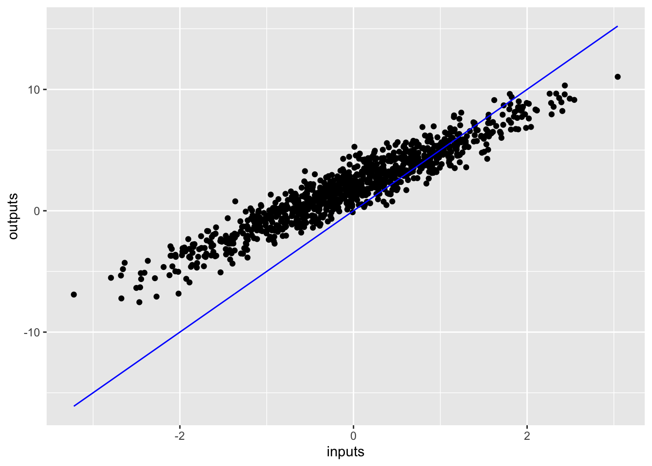
Define a training loop
With the network and training data, train the model using gradient descent to update the weights variable (W) and the bias variable (b) to reduce the loss.
There are many variants of the gradient descent scheme that are captured in tf$train$Optimizer—our recommended implementation. But in the spirit of building from first principles, here you will implement the basic math yourself with the help of tf.GradientTape for automatic differentiation and tf.assign_sub for decrementing a value (which combines tf.assign and tf.sub):
train <- function(model, inputs, outputs, learning_rate) {
  with (tf$GradientTape() %as% t, {
    current_loss = loss(model$call(inputs), outputs)
  })

  d <- t$gradient(current_loss, list(model$W, model$b))

  model$W$assign_sub(learning_rate * d[[1]])
  model$b$assign_sub(learning_rate * d[[2]])
  current_loss
}
Finally, let’s repeatedly run through the training data and see how W and b evolve.
model <- Model$new()

Ws <- bs <- c()

for (epoch in seq_len(20)) {

  Ws[epoch] <- as.numeric(model$W)
  bs[epoch] <- as.numeric(model$b)

  current_loss <- train(model, inputs, outputs, learning_rate = 0.1)
  cat(glue::glue("Epoch: {epoch}, Loss: {as.numeric(current_loss)}"), "\n")
}
## Epoch: 1, Loss: 9.22420692443848
## Epoch: 2, Loss: 6.19532537460327
## Epoch: 3, Loss: 4.27906942367554
## Epoch: 4, Loss: 3.06672716140747
## Epoch: 5, Loss: 2.29972267150879
## Epoch: 6, Loss: 1.81446659564972
## Epoch: 7, Loss: 1.50746238231659
## Epoch: 8, Loss: 1.31323146820068
## Epoch: 9, Loss: 1.19034790992737
## Epoch: 10, Loss: 1.11260342597961
## Epoch: 11, Loss: 1.06341695785522
## Epoch: 12, Loss: 1.03229808807373
## Epoch: 13, Loss: 1.01261019706726
## Epoch: 14, Loss: 1.0001540184021
## Epoch: 15, Loss: 0.992273688316345
## Epoch: 16, Loss: 0.987287759780884
## Epoch: 17, Loss: 0.984133422374725
## Epoch: 18, Loss: 0.982137799263
## Epoch: 19, Loss: 0.9808748960495
## Epoch: 20, Loss: 0.980076193809509tibble(
epoch = 1:20,
Ws = Ws,
bs = bs
) %>%
pivot_longer(
c(Ws, bs),
names_to = "parameter",
values_to = "estimate"
) %>%
ggplot(aes(x = epoch, y = estimate)) +
geom_line() +
facet_wrap(~parameter, scales = "free")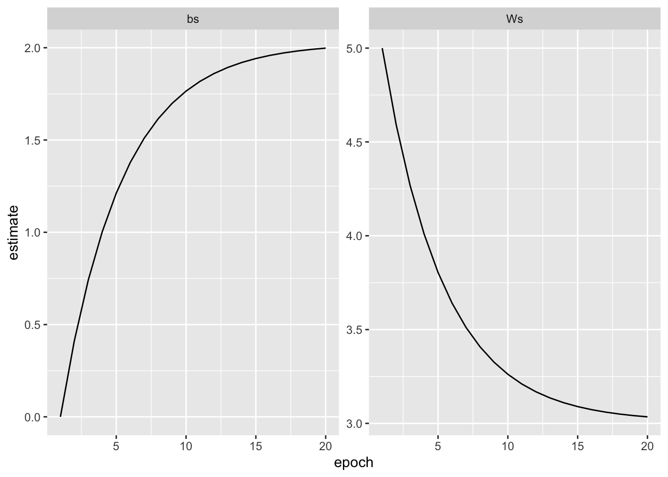
This tutorial used tf$Variable to build and train a simple linear model.
In practice, the high-level APIs—such as Keras—are much more convenient to build neural networks. Keras provides higher level building blocks (called “layers”), utilities to save and restore state, a suite of loss functions, a suite of optimization strategies, and more.