Convolutional Neural Network (CNN)
This tutorial demonstrates training a simple Convolutional Neural Network (CNN) to classify CIFAR images. Because this tutorial uses the Keras Sequential API, creating and training our model will take just a few lines of code.
Download and prepare the CIFAR10 dataset
The CIFAR10 dataset contains 60,000 color images in 10 classes, with 6,000 images in each class. The dataset is divided into 50,000 training images and 10,000 testing images. The classes are mutually exclusive and there is no overlap between them.
Verify the data
To verify that the dataset looks correct, let’s plot the first 25 images from the training set and display the class name below each image.
class_names <- c('airplane', 'automobile', 'bird', 'cat', 'deer',
               'dog', 'frog', 'horse', 'ship', 'truck')

index <- 1:30

par(mfcol = c(5,6), mar = rep(1, 4), oma = rep(0.2, 4))
cifar$train$x[index,,,] %>%
  purrr::array_tree(1) %>%
  purrr::set_names(class_names[cifar$train$y[index] + 1]) %>%
  purrr::map(as.raster, max = 255) %>%
  purrr::iwalk(~{plot(.x); title(.y)})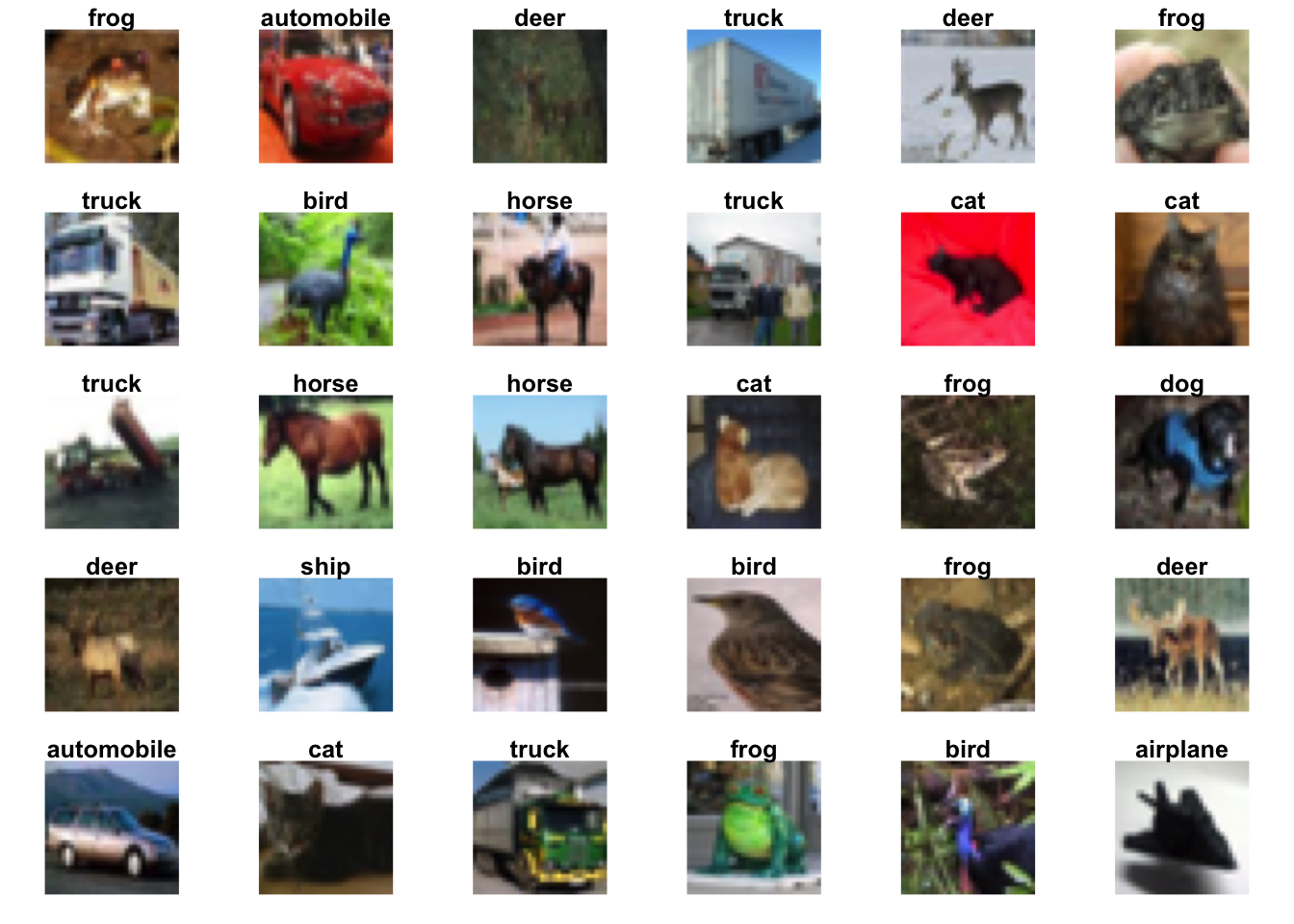
Create the convolutional base
The 6 lines of code below define the convolutional base using a common pattern: a stack of Conv2D and MaxPooling2D layers.
As input, a CNN takes tensors of shape (image_height, image_width, color_channels), ignoring the batch size. If you are new to these dimensions, color_channels refers to (R,G,B). In this example, you will configure our CNN to process inputs of shape (32, 32, 3), which is the format of CIFAR images. You can do this by passing the argument input_shape to our first layer.
model <- keras_model_sequential() %>%
  layer_conv_2d(filters = 32, kernel_size = c(3,3), activation = "relu",
                input_shape = c(32,32,3)) %>%
  layer_max_pooling_2d(pool_size = c(2,2)) %>%
  layer_conv_2d(filters = 64, kernel_size = c(3,3), activation = "relu") %>%
  layer_max_pooling_2d(pool_size = c(2,2)) %>%
  layer_conv_2d(filters = 64, kernel_size = c(3,3), activation = "relu")
Let’s display the architecture of our model so far.
## Model: "sequential"
## ___________________________________________________________________________
## Layer (type)                     Output Shape                  Param #
## ===========================================================================
## conv2d (Conv2D)                  (None, 30, 30, 32)            896
## ___________________________________________________________________________
## max_pooling2d (MaxPooling2D)     (None, 15, 15, 32)            0
## ___________________________________________________________________________
## conv2d_1 (Conv2D)                (None, 13, 13, 64)            18496
## ___________________________________________________________________________
## max_pooling2d_1 (MaxPooling2D)   (None, 6, 6, 64)              0
## ___________________________________________________________________________
## conv2d_2 (Conv2D)                (None, 4, 4, 64)              36928
## ===========================================================================
## Total params: 56,320
## Trainable params: 56,320
## Non-trainable params: 0
## ___________________________________________________________________________
Above, you can see that the output of every Conv2D and MaxPooling2D layer is a 3D tensor of shape (height, width, channels). The width and height dimensions tend to shrink as you go deeper in the network. The number of output channels for each Conv2D layer is controlled by the first argument (e.g., 32 or 64). Typically, as the width and height shrink, you can afford (computationally) to add more output channels in each Conv2D layer.
Add Dense layers on top
To complete our model, you will feed the last output tensor from the convolutional base (of shape (3, 3, 64)) into one or more Dense layers to perform classification. Dense layers take vectors as input (which are 1D), while the current output is a 3D tensor. First, you will flatten (or unroll) the 3D output to 1D, then add one or more Dense layers on top. CIFAR has 10 output classes, so you use a final Dense layer with 10 outputs and a softmax activation.
model %>%
  layer_flatten() %>%
  layer_dense(units = 64, activation = "relu") %>%
  layer_dense(units = 10, activation = "softmax")
Here’s the complete architecture of our model.
Note Keras models are mutable objects and you don’t need to re-assign model in the chubnk above.
## Model: "sequential"
## ___________________________________________________________________________
## Layer (type)                     Output Shape                  Param #
## ===========================================================================
## conv2d (Conv2D)                  (None, 30, 30, 32)            896
## ___________________________________________________________________________
## max_pooling2d (MaxPooling2D)     (None, 15, 15, 32)            0
## ___________________________________________________________________________
## conv2d_1 (Conv2D)                (None, 13, 13, 64)            18496
## ___________________________________________________________________________
## max_pooling2d_1 (MaxPooling2D)   (None, 6, 6, 64)              0
## ___________________________________________________________________________
## conv2d_2 (Conv2D)                (None, 4, 4, 64)              36928
## ___________________________________________________________________________
## flatten (Flatten)                (None, 1024)                  0
## ___________________________________________________________________________
## dense (Dense)                    (None, 64)                    65600
## ___________________________________________________________________________
## dense_1 (Dense)                  (None, 10)                    650
## ===========================================================================
## Total params: 122,570
## Trainable params: 122,570
## Non-trainable params: 0
## ___________________________________________________________________________
As you can see, our (3, 3, 64) outputs were flattened into vectors of shape (576) before going through two Dense layers.
Compile and train the model
model %>% compile(
optimizer = "adam",
loss = "sparse_categorical_crossentropy",
metrics = "accuracy"
)
history <- model %>%
fit(
x = cifar$train$x, y = cifar$train$y,
epochs = 10,
validation_data = unname(cifar$test),
verbose = 2
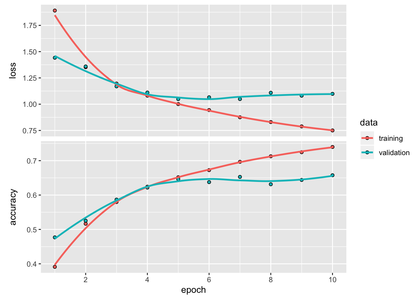
)## Train on 50000 samples, validate on 10000 samples
## Epoch 1/10
## 50000/50000 - 33s - loss: 1.8909 - accuracy: 0.3912 - val_loss: 1.4419 - val_accuracy: 0.4769
## Epoch 2/10
## 50000/50000 - 31s - loss: 1.3519 - accuracy: 0.5165 - val_loss: 1.3589 - val_accuracy: 0.5253
## Epoch 3/10
## 50000/50000 - 32s - loss: 1.1962 - accuracy: 0.5797 - val_loss: 1.1695 - val_accuracy: 0.5867
## Epoch 4/10
## 50000/50000 - 34s - loss: 1.0811 - accuracy: 0.6243 - val_loss: 1.1108 - val_accuracy: 0.6217
## Epoch 5/10
## 50000/50000 - 34s - loss: 1.0010 - accuracy: 0.6516 - val_loss: 1.0483 - val_accuracy: 0.6463
## Epoch 6/10
## 50000/50000 - 33s - loss: 0.9441 - accuracy: 0.6725 - val_loss: 1.0655 - val_accuracy: 0.6376
## Epoch 7/10
## 50000/50000 - 33s - loss: 0.8754 - accuracy: 0.6966 - val_loss: 1.0486 - val_accuracy: 0.6528
## Epoch 8/10
## 50000/50000 - 33s - loss: 0.8300 - accuracy: 0.7127 - val_loss: 1.1089 - val_accuracy: 0.6313
## Epoch 9/10
## 50000/50000 - 33s - loss: 0.7887 - accuracy: 0.7246 - val_loss: 1.0807 - val_accuracy: 0.6439
## Epoch 10/10
## 50000/50000 - 34s - loss: 0.7503 - accuracy: 0.7398 - val_loss: 1.0982 - val_accuracy: 0.6576Evaluate the model
## $loss
## [1] 1.098242
##
## $accuracy
## [1] 0.6576
Our simple CNN has achieved a test accuracy of over 70%. Not bad for a few lines of code!