Transfer learning with TensorFlow Hub
TensorFlow Hub is a way to share pretrained model components. See the TensorFlow Module Hub for a searchable listing of pre-trained models. This tutorial demonstrates:
- How to use TensorFlow Hub Keras.
- How to do image classification using TensorFlow Hub.
- How to do simple transfer learning.
An ImageNet classifier
Download the classifier
Use layer_hub to load a mobilenet and wrap it up as a keras layer. Any TensorFlow 2 compatible image classifier URL from tfhub.dev will work here.
Run it on a single image
Download a single image to try the model on.
image_url <- "https://storage.googleapis.com/download.tensorflow.org/example_images/grace_hopper.jpg"

img <- pins::pin(image_url, name = "grace_hopper") %>%
  tensorflow::tf$io$read_file() %>%
  tensorflow::tf$image$decode_image(dtype = tf$float32) %>%
  tensorflow::tf$image$resize(size = image_shape[-3])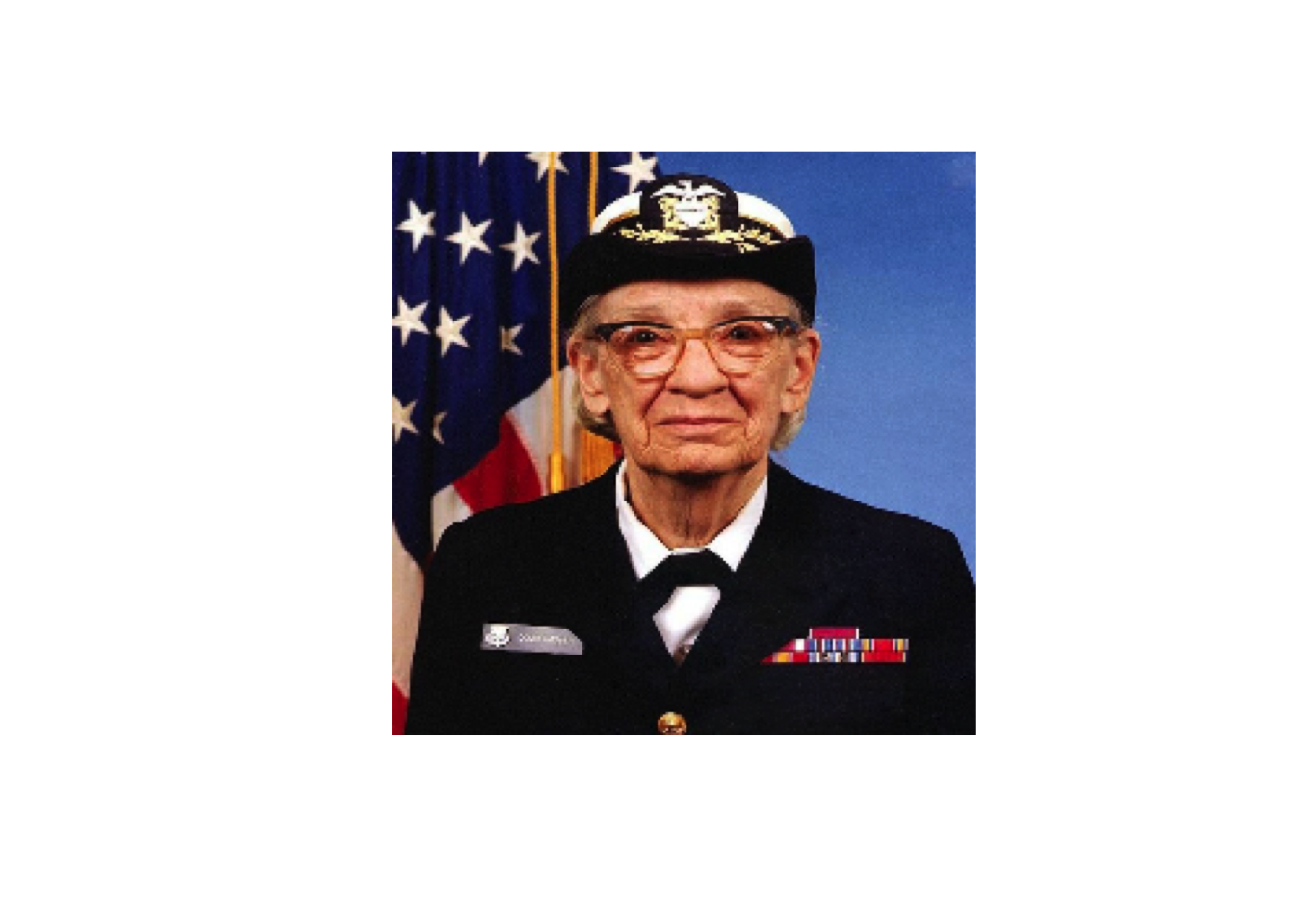
Add a batch dimension, and pass the image to the model.
The result is a 1001 element vector of logits, rating the probability of each class for the image.
So the top class ID can be found with argmax:
## [1] 653Decode the predictions
We have the predicted class ID, Fetch the ImageNet labels, and decode the predictions:
labels_url <- "https://storage.googleapis.com/download.tensorflow.org/data/ImageNetLabels.txt"

imagenet_labels <- pins::pin(labels_url, "imagenet_labels") %>%
  readLines()
img %>%
as.array() %>%
as.raster() %>%
plot()
#
title(paste("Prediction:" , imagenet_labels[predicted_class + 1]))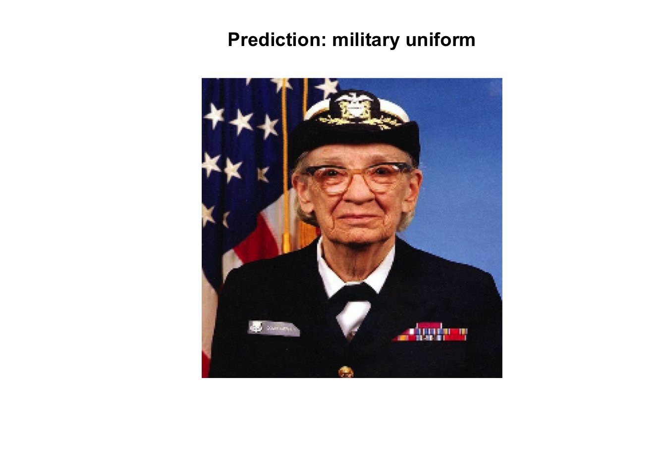
Simple transfer learning
Using TF Hub it is simple to retrain the top layer of the model to recognize the classes in our dataset.
flowers <- pins::pin("https://storage.googleapis.com/download.tensorflow.org/example_images/flower_photos.tgz", "flower_photos")The simplest way to load this data into our model is using image_data_generator.
All of TensorFlow Hub’s image modules expect float inputs in the [0, 1] range. Use the image_data_generator rescale parameter to achieve this.
The image size will be handled later.
image_generator <- image_data_generator(rescale=1/255)
image_data <- flowers[1] %>%
  dirname() %>%
  dirname() %>%
  flow_images_from_directory(image_generator, target_size = image_shape[-3])
## Found 3670 images belonging to 5 classes.The resulting object is an iterator that returns image_batch, label_batch pairs.
We can iterate over it using the iter_next from reticulate:
## List of 2
##  $ : num [1:32, 1:224, 1:224, 1:3] 0.145 0.431 0.431 0.863 1 ...
##  $ : num [1:32, 1:5] 1 0 0 0 0 0 0 0 0 0 ...
Run the classifier on a batch of images
Now run the classifier on the image batch.
image_batch <- reticulate::iter_next(image_data)
predictions <- classifier(tf$constant(image_batch[[1]], tf$float32))
predicted_classnames <- imagenet_labels[as.integer(tf$argmax(predictions, axis = 1L) + 1L)]par(mfcol = c(4,8), mar = rep(1, 4), oma = rep(0.2, 4))
image_batch[[1]] %>%
purrr::array_tree(1) %>%
purrr::set_names(predicted_classnames) %>%
purrr::map(as.raster) %>%
purrr::iwalk(~{plot(.x); title(.y)})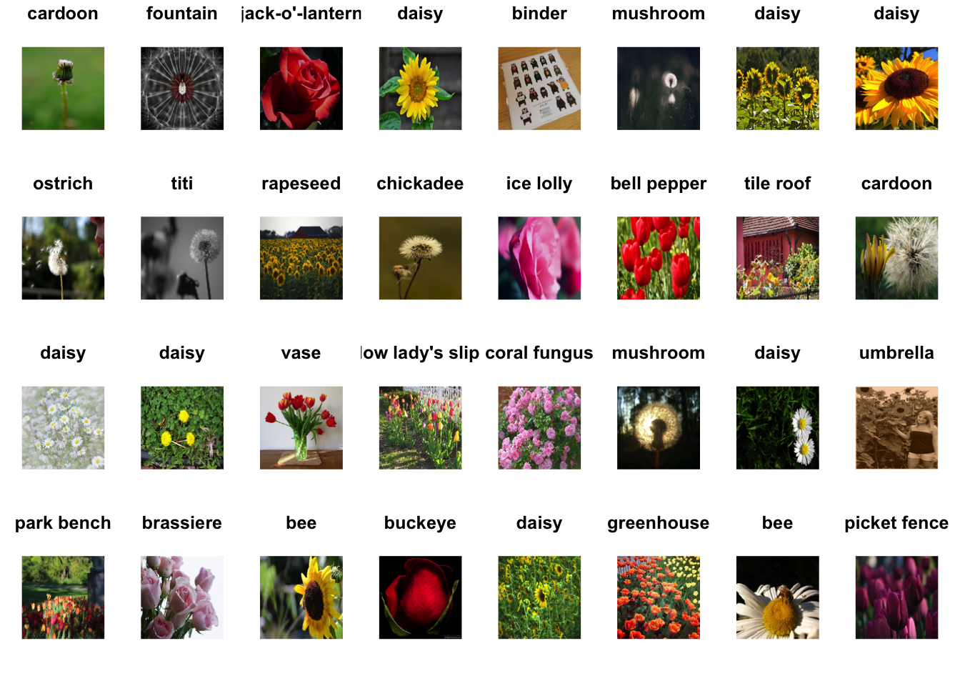
See the LICENSE.txt file for image attributions.
The results are far from perfect, but reasonable considering that these are not the classes the model was trained for (except “daisy”).
Download the headless model
TensorFlow Hub also distributes models without the top classification layer. These can be used to easily do transfer learning.
Any Tensorflow 2 compatible image feature vector URL from tfhub.dev will work here.
Create the feature extractor.
It returns a 1280-length vector for each image:
## tf.Tensor(
## [[0.13427277 0.16856195 0.283491   ... 0.00557477 0.         0.8134863 ]
##  [0.00754159 0.49517953 0.18708485 ... 0.01621983 0.         0.        ]
##  [0.         0.60116017 0.         ... 0.         0.05334444 0.00277256]
##  ...
##  [0.6140208  1.3715637  0.         ... 0.02907389 0.11318099 0.12228318]
##  [1.2423071  1.0235544  0.170658   ... 0.51680547 0.         0.        ]
##  [0.5452022  0.2789958  0.16163555 ... 0.1076004  0.01267634 0.        ]], shape=(32, 1280), dtype=float32)
Freeze the variables in the feature extractor layer, so that the training only modifies the new classifier layer.
Attach a classification head
Now let’s create a sequential model using the feature extraction layer and add a new classification layer.
model <- keras_model_sequential(list(
  feature_extractor_layer,
  layer_dense(units = image_data$num_classes, activation='softmax')
))

summary(model)
## Model: "sequential"
## ___________________________________________________________________________
## Layer (type) Output Shape Param #
## ===========================================================================
## keras_layer_1 (KerasLayer) (None, 1280) 2257984
## ___________________________________________________________________________
## dense (Dense) (None, 5) 6405
## ===========================================================================
## Total params: 2,264,389
## Trainable params: 6,405
## Non-trainable params: 2,257,984
## ___________________________________________________________________________Train the model
Use compile to configure the training process:
Now use the fit method to train the model.
To keep this example short train just 2 epochs.
history <- model %>% fit_generator(
  image_data, epochs=2,
  steps_per_epoch = image_data$n / image_data$batch_size,
  verbose = 2
)
## Epoch 1/2
## 114/114 - 255s - loss: 0.6656 - accuracy: 0.7567
## Epoch 2/2
## 114/114 - 250s - loss: 0.3308 - accuracy: 0.8931Now after, even just a few training iterations, we can already see that the model is making progress on the task.
We can then verify the predictions:
image_batch <- reticulate::iter_next(image_data)
predictions <- predict_classes(model, image_batch[[1]])

par(mfcol = c(4,8), mar = rep(1, 4), oma = rep(0.2, 4))
image_batch[[1]] %>%
  purrr::array_tree(1) %>%
  purrr::set_names(names(image_data$class_indices)[predictions + 1]) %>%
  purrr::map(as.raster) %>%
  purrr::iwalk(~{plot(.x); title(.y)})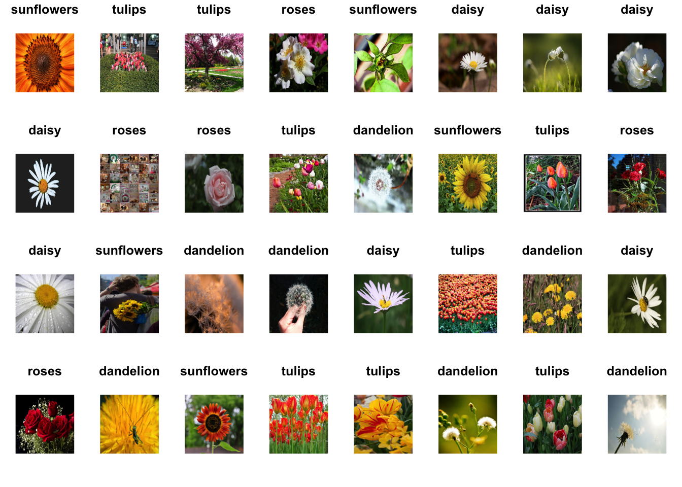
Export your model
Now that you’ve trained the model, export it as a saved model:
Now confirm that we can reload it, and it still gives the same results:
x <- tf$constant(image_batch[[1]], tf$float32)
all.equal(
  as.matrix(model(x)),
  as.matrix(model_(x))
)
## [1] TRUE