Classify structured data with feature columns

The Dataset

We will use a small dataset provided by the Cleveland Clinic Foundation for Heart Disease. There are several hundred rows in the CSV. Each row describes a patient, and each column describes an attribute. We will use this information to predict whether a patient has heart disease, which in this dataset is a binary classification task.

Following is a description of this dataset. Notice there are both numeric and categorical columns.

Column	Description	Feature Type	Data Type
Age	Age in years	Numerical	integer
Sex	(1 = male; 0 = female)	Categorical	integer
CP	Chest pain type (0, 1, 2, 3, 4)	Categorical	integer
Trestbpd	Resting blood pressure (in mm Hg on admission to the hospital)	Numerical	integer
Chol	Serum cholestoral in mg/dl	Numerical	integer
FBS	(fasting blood sugar > 120 mg/dl) (1 = true; 0 = false)	Categorical	integer
RestECG	Resting electrocardiographic results (0, 1, 2)	Categorical	integer
Thalach	Maximum heart rate achieved	Numerical	integer
Exang	Exercise induced angina (1 = yes; 0 = no)	Categorical	integer
Oldpeak	ST depression induced by exercise relative to rest	Numerical	integer
Slope	The slope of the peak exercise ST segment	Numerical	float
CA	Number of major vessels (0-3) colored by flourosopy	Numerical	integer
Thal	3 = normal; 6 = fixed defect; 7 = reversable defect	Categorical	string
Target	Diagnosis of heart disease (1 = true; 0 = false)	Classification	integer

Setup

We will use Keras and TensorFlow datasets.

library(keras)
library(tfdatasets)
library(tidyverse)

## ── Attaching packages ─────────────────────────────────────────────────────────────── tidyverse 1.2.1 ──

## ✔ ggplot2 3.2.0     ✔ purrr   0.3.2
## ✔ tibble  2.1.3     ✔ dplyr   0.8.3
## ✔ tidyr   1.0.0     ✔ stringr 1.4.0
## ✔ readr   1.3.1     ✔ forcats 0.4.0

## ── Conflicts ────────────────────────────────────────────────────────────────── tidyverse_conflicts() ──
## ✖ dplyr::filter() masks stats::filter()
## ✖ dplyr::lag()    masks stats::lag()

library(rsample)

Read the data

We will use read_csv in order to read the csv file to R.

heart <- pins::pin("https://storage.googleapis.com/applied-dl/heart.csv", "heart")
df <- read_csv(heart)

## Parsed with column specification:
## cols(
##   age = col_double(),
##   sex = col_double(),
##   cp = col_double(),
##   trestbps = col_double(),
##   chol = col_double(),
##   fbs = col_double(),
##   restecg = col_double(),
##   thalach = col_double(),
##   exang = col_double(),
##   oldpeak = col_double(),
##   slope = col_double(),
##   ca = col_double(),
##   thal = col_character(),
##   target = col_double()
## )

glimpse(df)

## Observations: 303
## Variables: 14
## $ age      <dbl> 63, 67, 67, 37, 41, 56, 62, 57, 63, 53, 57, 56, 56, 44,…
## $ sex      <dbl> 1, 1, 1, 1, 0, 1, 0, 0, 1, 1, 1, 0, 1, 1, 1, 1, 1, 1, 0…
## $ cp       <dbl> 1, 4, 4, 3, 2, 2, 4, 4, 4, 4, 4, 2, 3, 2, 3, 3, 2, 4, 3…
## $ trestbps <dbl> 145, 160, 120, 130, 130, 120, 140, 120, 130, 140, 140, …
## $ chol     <dbl> 233, 286, 229, 250, 204, 236, 268, 354, 254, 203, 192, …
## $ fbs      <dbl> 1, 0, 0, 0, 0, 0, 0, 0, 0, 1, 0, 0, 1, 0, 1, 0, 0, 0, 0…
## $ restecg  <dbl> 2, 2, 2, 0, 2, 0, 2, 0, 2, 2, 0, 2, 2, 0, 0, 0, 0, 0, 0…
## $ thalach  <dbl> 150, 108, 129, 187, 172, 178, 160, 163, 147, 155, 148, …
## $ exang    <dbl> 0, 1, 1, 0, 0, 0, 0, 1, 0, 1, 0, 0, 1, 0, 0, 0, 0, 0, 0…
## $ oldpeak  <dbl> 2.3, 1.5, 2.6, 3.5, 1.4, 0.8, 3.6, 0.6, 1.4, 3.1, 0.4, …
## $ slope    <dbl> 3, 2, 2, 3, 1, 1, 3, 1, 2, 3, 2, 2, 2, 1, 1, 1, 3, 1, 1…
## $ ca       <dbl> 0, 3, 2, 0, 0, 0, 2, 0, 1, 0, 0, 0, 1, 0, 0, 0, 0, 0, 0…
## $ thal     <chr> "fixed", "normal", "reversible", "normal", "normal", "n…
## $ target   <dbl> 0, 1, 0, 0, 0, 0, 1, 0, 1, 0, 0, 0, 1, 0, 0, 0, 0, 0, 0…

Split the dataframe into train, validation, and test

We are going to use the rsample package to split the data into train, validation and test sets.

# first we split between training and testing sets
split <- initial_split(df, prop = 4/5)
train <- training(split)
test <- testing(split)

# the we split the training set into validation and training
split <- initial_split(train, prop = 4/5)
train <- training(split)
val <- testing(split)

nrow(train)

## [1] 195

nrow(val)

## [1] 48

nrow(test)

## [1] 60

Create an input pipeline using tfdatasets

Next, we will wrap the dataframes with tfdatasets. This will enable us to use feature columns as a bridge to map from the columns in the dataframe to features used to train the model. If we were working with a very large CSV file (so large that it does not fit into memory), we would use tfdatasets to read it from disk directly. That is not covered in this tutorial.

df_to_dataset <- function(df, shuffle = TRUE, batch_size = 32) {
  ds <- df %>% 
    tensor_slices_dataset()
  
  if (shuffle)
    ds <- ds %>% dataset_shuffle(buffer_size = nrow(df))
  
  ds %>% 
    dataset_batch(batch_size = batch_size)
}

batch_size <- 5
train_ds <- df_to_dataset(train, batch_size = batch_size)
val_ds <- df_to_dataset(val, shuffle = FALSE, batch_size = batch_size)
test_ds <- df_to_dataset(test, shuffle = FALSE, batch_size = batch_size)

Understand the input pipeline

Now that we have created the input pipeline, let’s call it to see the format of the data it returns. We have used a small batch size to keep the output readable.

train_ds %>% 
  reticulate::as_iterator() %>% 
  reticulate::iter_next() %>% 
  str()

## List of 14
##  $ age     :tf.Tensor([54. 60. 52. 66. 54.], shape=(5,), dtype=float32)
##  $ sex     :tf.Tensor([0. 0. 1. 1. 1.], shape=(5,), dtype=float32)
##  $ cp      :tf.Tensor([2. 3. 4. 4. 4.], shape=(5,), dtype=float32)
##  $ trestbps:tf.Tensor([132. 102. 128. 112. 110.], shape=(5,), dtype=float32)
##  $ chol    :tf.Tensor([288. 318. 255. 212. 239.], shape=(5,), dtype=float32)
##  $ fbs     :tf.Tensor([1. 0. 0. 0. 0.], shape=(5,), dtype=float32)
##  $ restecg :tf.Tensor([2. 0. 0. 2. 0.], shape=(5,), dtype=float32)
##  $ thalach :tf.Tensor([159. 160. 161. 132. 126.], shape=(5,), dtype=float32)
##  $ exang   :tf.Tensor([1. 0. 1. 1. 1.], shape=(5,), dtype=float32)
##  $ oldpeak :tf.Tensor([0.  0.  0.  0.1 2.8], shape=(5,), dtype=float32)
##  $ slope   :tf.Tensor([1. 1. 1. 1. 2.], shape=(5,), dtype=float32)
##  $ ca      :tf.Tensor([1. 1. 1. 1. 1.], shape=(5,), dtype=float32)
##  $ thal    :tf.Tensor([b'normal' b'normal' b'reversible' b'normal' b'reversible'], shape=(5,), dtype=string)
##  $ target  :tf.Tensor([0. 0. 0. 1. 1.], shape=(5,), dtype=float32)

We can see that the dataset returns a list of column names (from the dataframe) that map to column values from rows in the dataframe.

Create the feature spec

We want to train a model to predict the target variable using Keras but, before that we need to prepare the data. We need to transform the categorical variables into some form of dense variable, we usually want to normalize all numeric columns too.

The feature spec interface works with data.frames or TensorFlow datasets objects.

Let’s start creating our feature specification:

spec <- feature_spec(train_ds, target ~ .)

The first thing we need to do after creating the feature_spec is decide on the variables’ types.

We can do this by adding steps to the spec object.

spec <- spec %>% 
  step_numeric_column(
    all_numeric(), -cp, -restecg, -exang, -sex, -fbs,
    normalizer_fn = scaler_standard()
  ) %>% 
  step_categorical_column_with_vocabulary_list(thal)

The following steps can be used to define the variable type:

• step_numeric_column to define numeric variables
• step_categorical_with_vocabulary_list for categorical variables with a fixed vocabulary
• step_categorical_column_with_hash_bucket for categorical variables using the hash trick
• step_categorical_column_with_identity to store categorical variables as integers
• step_categorical_column_with_vocabulary_file when you have the possible vocabulary in a file

When using step_categorical_column_with_vocabulary_list you can also provide a vocabulary argument with the fixed vocabulary. The recipe will find all the unique values in the dataset and use it as the vocabulary.

You can also specify a normalizer_fn to the step_numeric_column. In this case the variable will be transformed by the feature column. Note that the transformation will occur in the TensorFlow Graph, so it must use only TensorFlow ops. Like in the example we offer pre-made normalizers - and they will compute the normalizing function during the recipe preparation.

You can also use selectors like:

• starts_with(), ends_with(), matches() etc. (from tidyselect)
• all_numeric() to select all numeric variables
• all_nominal() to select all strings
• has_type("float32") to select based on TensorFlow variable type.

Now we can print the recipe:

spec

## ── Feature Spec ──────────────────────────────────────────────────────────────────────────────────────── 
## A feature_spec with 8 steps.
## Fitted: FALSE 
## ── Steps ─────────────────────────────────────────────────────────────────────────────────────────────── 
## StepCategoricalColumnWithVocabularyList: thal 
## StepNumericColumn: age, trestbps, chol, thalach, oldpeak, slope, ca 
## ── Dense features ────────────────────────────────────────────────────────────────────────────────────── 
## Feature spec must be fitted before we can detect the dense features.

After specifying the types of the columns you can add transformation steps. For example you may want to bucketize a numeric column:

spec <- spec %>% 
  step_bucketized_column(age, boundaries = c(18, 25, 30, 35, 40, 45, 50, 55, 60, 65))

You can also specify the kind of numeric representation that you want to use for your categorical variables.

spec <- spec %>% 
  step_indicator_column(thal) %>% 
  step_embedding_column(thal, dimension = 2)

Another common transformation is to add interactions between variables using crossed columns.

spec <- spec %>% 
  step_crossed_column(thal_and_age = c(thal, bucketized_age), hash_bucket_size = 1000) %>% 
  step_indicator_column(thal_and_age)

Note that the crossed_column is a categorical column, so we need to also specify what kind of numeric tranformation we want to use. Also note that we can name the transformed variables - each step uses a default naming for columns, eg. bucketized_age is the default name when you use step_bucketized_column with column called age.

With the above code we have created our recipe. Note we can also define the recipe by chaining a sequence of methods:

spec <- feature_spec(train_ds, target ~ .) %>% 
  step_numeric_column(
    all_numeric(), -cp, -restecg, -exang, -sex, -fbs,
    normalizer_fn = scaler_standard()
  ) %>% 
  step_categorical_column_with_vocabulary_list(thal) %>% 
  step_bucketized_column(age, boundaries = c(18, 25, 30, 35, 40, 45, 50, 55, 60, 65)) %>% 
  step_indicator_column(thal) %>% 
  step_embedding_column(thal, dimension = 2) %>% 
  step_crossed_column(c(thal, bucketized_age), hash_bucket_size = 10) %>%
  step_indicator_column(crossed_thal_bucketized_age)

After defining the recipe we need to fit it. It’s when fitting that we compute the vocabulary list for categorical variables or find the mean and standard deviation for the normalizing functions. Fitting involves evaluating the full dataset, so if you have provided the vocabulary list and your columns are already normalized you can skip the fitting step (TODO).

In our case, we will fit the feature spec, since we didn’t specify the vocabulary list for the categorical variables.

spec_prep <- fit(spec)

After preparing we can see the list of dense features that were defined:

str(spec_prep$dense_features())

## List of 11
##  $ age                                  :NumericColumn(key='age', shape=(1,), default_value=None, dtype=tf.float32, normalizer_fn=<function make_python_function.<locals>.python_function at 0x136510ea0>)
##  $ trestbps                             :NumericColumn(key='trestbps', shape=(1,), default_value=None, dtype=tf.float32, normalizer_fn=<function make_python_function.<locals>.python_function at 0x1311f2ea0>)
##  $ chol                                 :NumericColumn(key='chol', shape=(1,), default_value=None, dtype=tf.float32, normalizer_fn=<function make_python_function.<locals>.python_function at 0x1311f2158>)
##  $ thalach                              :NumericColumn(key='thalach', shape=(1,), default_value=None, dtype=tf.float32, normalizer_fn=<function make_python_function.<locals>.python_function at 0x1311f2f28>)
##  $ oldpeak                              :NumericColumn(key='oldpeak', shape=(1,), default_value=None, dtype=tf.float32, normalizer_fn=<function make_python_function.<locals>.python_function at 0x1311ec048>)
##  $ slope                                :NumericColumn(key='slope', shape=(1,), default_value=None, dtype=tf.float32, normalizer_fn=<function make_python_function.<locals>.python_function at 0x1311ec0d0>)
##  $ ca                                   :NumericColumn(key='ca', shape=(1,), default_value=None, dtype=tf.float32, normalizer_fn=<function make_python_function.<locals>.python_function at 0x1311ec158>)
##  $ bucketized_age                       :BucketizedColumn(source_column=NumericColumn(key='age', shape=(1,), default_value=None, dtype=tf.float32, normalizer_fn=<function make_python_function.<locals>.python_function at 0x136510ea0>), boundaries=(18.0, 25.0, 30.0, 35.0, 40.0, 45.0, 50.0, 55.0, 60.0, 65.0))
##  $ indicator_thal                       :IndicatorColumn(categorical_column=VocabularyListCategoricalColumn(key='thal', vocabulary_list=('fixed', 'normal', 'reversible'), dtype=tf.string, default_value=-1, num_oov_buckets=0))
##  $ embedding_thal                       :EmbeddingColumn(categorical_column=VocabularyListCategoricalColumn(key='thal', vocabulary_list=('fixed', 'normal', 'reversible'), dtype=tf.string, default_value=-1, num_oov_buckets=0), dimension=2, combiner='mean', initializer=<tensorflow.python.ops.init_ops.TruncatedNormal>, ckpt_to_load_from=None, tensor_name_in_ckpt=None, max_norm=None, trainable=True)
##  $ indicator_crossed_thal_bucketized_age:IndicatorColumn(categorical_column=CrossedColumn(keys=(VocabularyListCategoricalColumn(key='thal', vocabulary_list=('fixed', 'normal', 'reversible'), dtype=tf.string, default_value=-1, num_oov_buckets=0), BucketizedColumn(source_column=NumericColumn(key='age', shape=(1,), default_value=None, dtype=tf.float32, normalizer_fn=<function make_python_function.<locals>.python_function at 0x136510ea0>), boundaries=(18.0, 25.0, 30.0, 35.0, 40.0, 45.0, 50.0, 55.0, 60.0, 65.0))), hash_bucket_size=10.0, hash_key=None))

Build the model

Now we are ready to define our model in Keras. We will use a specialized layer_dense_features that knows what to do with the feature columns specification.

We also use a new layer_input_from_dataset that is useful to create a Keras input object copying the structure from a data.frame or TensorFlow dataset.

model <- keras_model_sequential() %>% 
  layer_dense_features(dense_features(spec_prep)) %>% 
  layer_dense(units = 32, activation = "relu") %>% 
  layer_dense(units = 1, activation = "sigmoid")


model %>% compile(
  loss = loss_binary_crossentropy, 
  optimizer = "adam", 
  metrics = "binary_accuracy"
)

Train the model

We can finally train the model on the dataset:

history <- model %>% 
  fit(
    dataset_use_spec(train_ds, spec = spec_prep),
    epochs = 15, 
    validation_data = dataset_use_spec(val_ds, spec_prep),
    verbose = 2
  )

## Epoch 1/15
## 39/39 - 1s - loss: 0.6738 - binary_accuracy: 0.6513 - val_loss: 0.0000e+00 - val_binary_accuracy: 0.0000e+00
## Epoch 2/15
## 39/39 - 0s - loss: 0.5535 - binary_accuracy: 0.7692 - val_loss: 0.5300 - val_binary_accuracy: 0.7708
## Epoch 3/15
## 39/39 - 0s - loss: 0.4731 - binary_accuracy: 0.8103 - val_loss: 0.4800 - val_binary_accuracy: 0.7917
## Epoch 4/15
## 39/39 - 0s - loss: 0.4254 - binary_accuracy: 0.8359 - val_loss: 0.4566 - val_binary_accuracy: 0.7917
## Epoch 5/15
## 39/39 - 0s - loss: 0.3922 - binary_accuracy: 0.8410 - val_loss: 0.4395 - val_binary_accuracy: 0.8125
## Epoch 6/15
## 39/39 - 0s - loss: 0.3678 - binary_accuracy: 0.8564 - val_loss: 0.4326 - val_binary_accuracy: 0.7917
## Epoch 7/15
## 39/39 - 0s - loss: 0.3600 - binary_accuracy: 0.8615 - val_loss: 0.4208 - val_binary_accuracy: 0.8125
## Epoch 8/15
## 39/39 - 0s - loss: 0.3469 - binary_accuracy: 0.8615 - val_loss: 0.4167 - val_binary_accuracy: 0.7917
## Epoch 9/15
## 39/39 - 0s - loss: 0.3404 - binary_accuracy: 0.8615 - val_loss: 0.4076 - val_binary_accuracy: 0.7917
## Epoch 10/15
## 39/39 - 0s - loss: 0.3308 - binary_accuracy: 0.8667 - val_loss: 0.4115 - val_binary_accuracy: 0.7917
## Epoch 11/15
## 39/39 - 0s - loss: 0.3109 - binary_accuracy: 0.8615 - val_loss: 0.4136 - val_binary_accuracy: 0.7917
## Epoch 12/15
## 39/39 - 0s - loss: 0.3239 - binary_accuracy: 0.8667 - val_loss: 0.4033 - val_binary_accuracy: 0.7917
## Epoch 13/15
## 39/39 - 0s - loss: 0.3176 - binary_accuracy: 0.8564 - val_loss: 0.4046 - val_binary_accuracy: 0.7917
## Epoch 14/15
## 39/39 - 0s - loss: 0.3171 - binary_accuracy: 0.8615 - val_loss: 0.3979 - val_binary_accuracy: 0.7917
## Epoch 15/15
## 39/39 - 0s - loss: 0.3040 - binary_accuracy: 0.8615 - val_loss: 0.3967 - val_binary_accuracy: 0.7917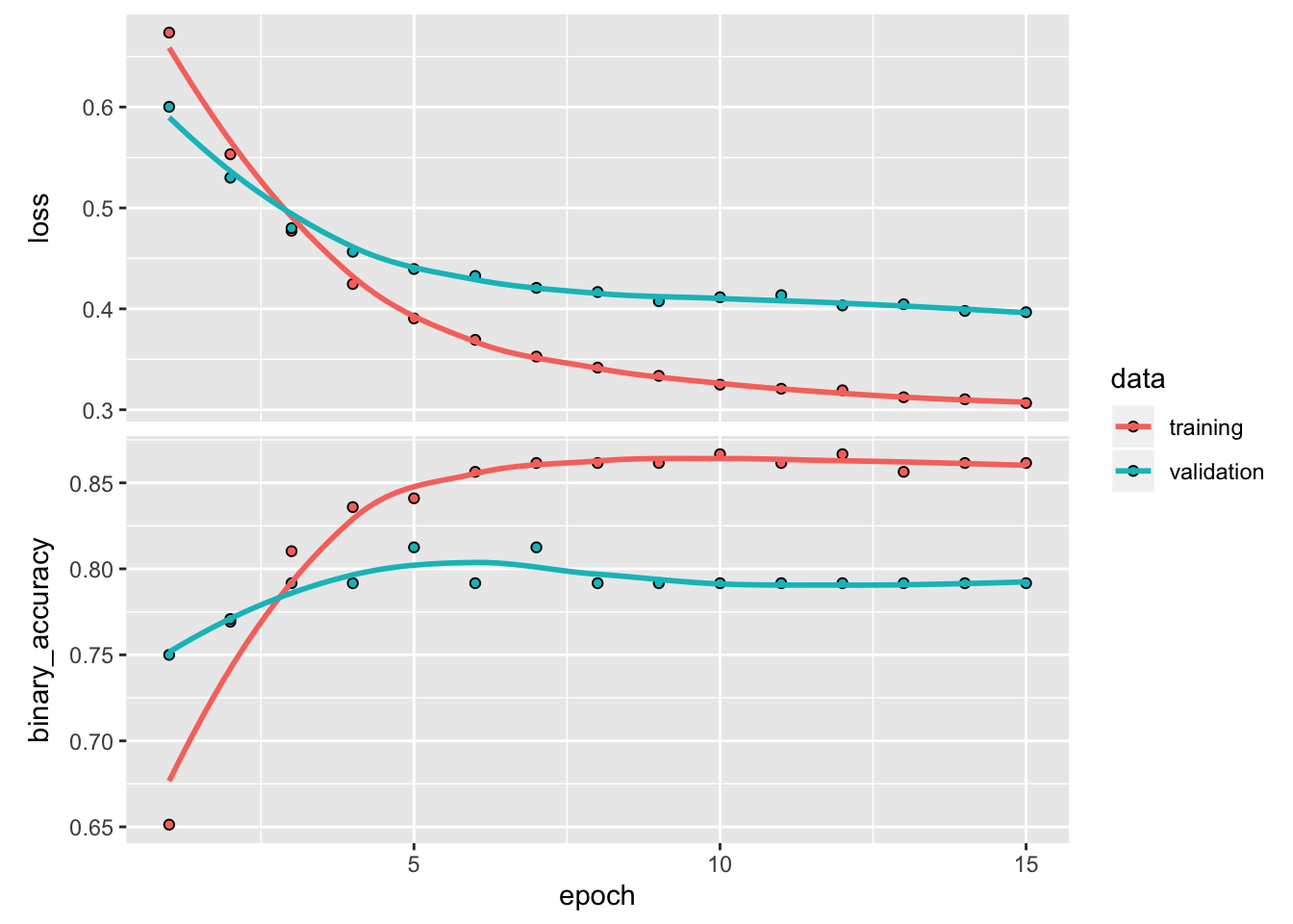

plot(history)

Finally we can make predictions in the test set and calculate performance metrics like the AUC of the ROC curve:

pred <- predict(model, test)
Metrics::auc(test$target, pred)

## [1] 0.890538