Basic Regression

In a regression problem, we aim to predict the output of a continuous value, like a price or a probability. Contrast this with a classification problem, where we aim to predict a discrete label (for example, where a picture contains an apple or an orange).

This notebook builds a model to predict the median price of homes in a Boston suburb during the mid-1970s. To do this, we’ll provide the model with some data points about the suburb, such as the crime rate and the local property tax rate.

library(keras)
library(tfdatasets)

The Boston Housing Prices dataset

The Boston Housing Prices dataset is accessible directly from keras.

boston_housing <- dataset_boston_housing()

c(train_data, train_labels) %<-% boston_housing$train
c(test_data, test_labels) %<-% boston_housing$test

Examples and features

This dataset is much smaller than the others we’ve worked with so far: it has 506 total examples that are split between 404 training examples and 102 test examples:

paste0("Training entries: ", length(train_data), ", labels: ", length(train_labels))

## [1] "Training entries: 5252, labels: 404"

The dataset contains 13 different features:

Per capita crime rate.
The proportion of residential land zoned for lots over 25,000 square feet.
The proportion of non-retail business acres per town.
Charles River dummy variable (= 1 if tract bounds river; 0 otherwise).
Nitric oxides concentration (parts per 10 million).
The average number of rooms per dwelling.
The proportion of owner-occupied units built before 1940.
Weighted distances to five Boston employment centers.
Index of accessibility to radial highways.
Full-value property-tax rate per $10,000.
Pupil-teacher ratio by town.
1000 * (Bk - 0.63) ** 2 where Bk is the proportion of Black people by town.
Percentage lower status of the population.

Each one of these input data features is stored using a different scale. Some features are represented by a proportion between 0 and 1, other features are ranges between 1 and 12, some are ranges between 0 and 100, and so on.

train_data[1, ] # Display sample features, notice the different scales

##  [1]   1.23247   0.00000   8.14000   0.00000   0.53800   6.14200  91.70000
##  [8]   3.97690   4.00000 307.00000  21.00000 396.90000  18.72000

Let’s add column names for better data inspection.

library(dplyr)

column_names <- c('CRIM', 'ZN', 'INDUS', 'CHAS', 'NOX', 'RM', 'AGE', 
                  'DIS', 'RAD', 'TAX', 'PTRATIO', 'B', 'LSTAT')

train_df <- train_data %>% 
  as_tibble(.name_repair = "minimal") %>% 
  setNames(column_names) %>% 
  mutate(label = train_labels)

test_df <- test_data %>% 
  as_tibble(.name_repair = "minimal") %>% 
  setNames(column_names) %>% 
  mutate(label = test_labels)

Labels

The labels are the house prices in thousands of dollars. (You may notice the mid-1970s prices.)

train_labels[1:10] # Display first 10 entries

##  [1] 15.2 42.3 50.0 21.1 17.7 18.5 11.3 15.6 15.6 14.4

Normalize features

It’s recommended to normalize features that use different scales and ranges. Although the model might converge without feature normalization, it makes training more difficult, and it makes the resulting model more dependent on the choice of units used in the input.

We are going to use the feature_spec interface implemented in the tfdatasets package for normalization. The feature_columns interface allows for other common pre-processing operations on tabular data.

spec <- feature_spec(train_df, label ~ . ) %>% 
  step_numeric_column(all_numeric(), normalizer_fn = scaler_standard()) %>% 
  fit()

spec

## ── Feature Spec ─────────────────────────────────────────────────────────────────────────── 
## A feature_spec with 13 steps.
## Fitted: TRUE 
## ── Steps ────────────────────────────────────────────────────────────────────────────────── 
## The feature_spec has 1 dense features.
## StepNumericColumn: CRIM, ZN, INDUS, CHAS, NOX, RM, AGE, DIS, RAD, TAX, PTRATIO, B, LSTAT 
## ── Dense features ─────────────────────────────────────────────────────────────────────────

The spec created with tfdatasets can be used together with layer_dense_features to perform pre-processing directly in the TensorFlow graph.

We can take a look at the output of a dense-features layer created by this spec:

layer <- layer_dense_features(
  feature_columns = dense_features(spec), 
  dtype = tf$float32
)
layer(train_df)

## tf.Tensor(
## [[ 0.81205493  0.44752213 -0.2565147  ... -0.1762239  -0.59443307
##   -0.48301655]
##  [-1.9079947   0.43137115 -0.2565147  ...  1.8920003  -0.34800112
##    2.9880793 ]
##  [ 1.1091131   0.2203439  -0.2565147  ... -1.8274226   1.563349
##   -0.48301655]
##  ...
##  [-1.6359899   0.07934052 -0.2565147  ... -0.3326088  -0.61246467
##    0.9895695 ]
##  [ 1.0554279  -0.98642045 -0.2565147  ... -0.7862657  -0.01742171
##   -0.48301655]
##  [-1.7970455   0.23288251 -0.2565147  ...  0.47467488 -0.84687555
##    2.0414166 ]], shape=(404, 13), dtype=float32)

Note that this returns a matrix (in the sense that it’s a 2-dimensional Tensor) with scaled values.

Create the model

Let’s build our model. Here we will use the Keras functional API - which is the recommended way when using the feature_spec API. Note that we only need to pass the dense_features from the spec we just created.

input <- layer_input_from_dataset(train_df %>% select(-label))

output <- input %>% 
  layer_dense_features(dense_features(spec)) %>% 
  layer_dense(units = 64, activation = "relu") %>%
  layer_dense(units = 64, activation = "relu") %>%
  layer_dense(units = 1) 

model <- keras_model(input, output)

summary(model)

## Model: "model"
## ___________________________________________________________________________
## Layer (type)            Output Shape     Param #  Connected to             
## ===========================================================================
## AGE (InputLayer)        [(None,)]        0                                 
## ___________________________________________________________________________
## B (InputLayer)          [(None,)]        0                                 
## ___________________________________________________________________________
## CHAS (InputLayer)       [(None,)]        0                                 
## ___________________________________________________________________________
## CRIM (InputLayer)       [(None,)]        0                                 
## ___________________________________________________________________________
## DIS (InputLayer)        [(None,)]        0                                 
## ___________________________________________________________________________
## INDUS (InputLayer)      [(None,)]        0                                 
## ___________________________________________________________________________
## LSTAT (InputLayer)      [(None,)]        0                                 
## ___________________________________________________________________________
## NOX (InputLayer)        [(None,)]        0                                 
## ___________________________________________________________________________
## PTRATIO (InputLayer)    [(None,)]        0                                 
## ___________________________________________________________________________
## RAD (InputLayer)        [(None,)]        0                                 
## ___________________________________________________________________________
## RM (InputLayer)         [(None,)]        0                                 
## ___________________________________________________________________________
## TAX (InputLayer)        [(None,)]        0                                 
## ___________________________________________________________________________
## ZN (InputLayer)         [(None,)]        0                                 
## ___________________________________________________________________________
## dense_features_1 (Dense (None, 13)       0        AGE[0][0]                
##                                                   B[0][0]                  
##                                                   CHAS[0][0]               
##                                                   CRIM[0][0]               
##                                                   DIS[0][0]                
##                                                   INDUS[0][0]              
##                                                   LSTAT[0][0]              
##                                                   NOX[0][0]                
##                                                   PTRATIO[0][0]            
##                                                   RAD[0][0]                
##                                                   RM[0][0]                 
##                                                   TAX[0][0]                
##                                                   ZN[0][0]                 
## ___________________________________________________________________________
## dense (Dense)           (None, 64)       896      dense_features_1[0][0]   
## ___________________________________________________________________________
## dense_1 (Dense)         (None, 64)       4160     dense[0][0]              
## ___________________________________________________________________________
## dense_2 (Dense)         (None, 1)        65       dense_1[0][0]            
## ===========================================================================
## Total params: 5,121
## Trainable params: 5,121
## Non-trainable params: 0
## ___________________________________________________________________________

We then compile the model with:

model %>% 
  compile(
    loss = "mse",
    optimizer = optimizer_rmsprop(),
    metrics = list("mean_absolute_error")
  )

We will wrap the model building code into a function in order to be able to reuse it for different experiments. Remember that Keras fit modifies the model in-place.

build_model <- function() {
  input <- layer_input_from_dataset(train_df %>% select(-label))
  
  output <- input %>% 
    layer_dense_features(dense_features(spec)) %>% 
    layer_dense(units = 64, activation = "relu") %>%
    layer_dense(units = 64, activation = "relu") %>%
    layer_dense(units = 1) 
  
  model <- keras_model(input, output)
  
  model %>% 
    compile(
      loss = "mse",
      optimizer = optimizer_rmsprop(),
      metrics = list("mean_absolute_error")
    )
  
  model
}

Train the model

The model is trained for 500 epochs, recording training and validation accuracy in a keras_training_history object. We also show how to use a custom callback, replacing the default training output by a single dot per epoch.

# Display training progress by printing a single dot for each completed epoch.
print_dot_callback <- callback_lambda(
  on_epoch_end = function(epoch, logs) {
    if (epoch %% 80 == 0) cat("\n")
    cat(".")
  }
)    

model <- build_model()

history <- model %>% fit(
  x = train_df %>% select(-label),
  y = train_df$label,
  epochs = 500,
  validation_split = 0.2,
  verbose = 0,
  callbacks = list(print_dot_callback)
)

## 
## ................................................................................
## ................................................................................
## ................................................................................
## ................................................................................
## ................................................................................
## ................................................................................
## ....................

Now, we visualize the model’s training progress using the metrics stored in the history variable. We want to use this data to determine how long to train before the model stops making progress.

library(ggplot2)

## 
## Attaching package: 'ggplot2'

## The following object is masked _by_ '.GlobalEnv':
## 
##     layer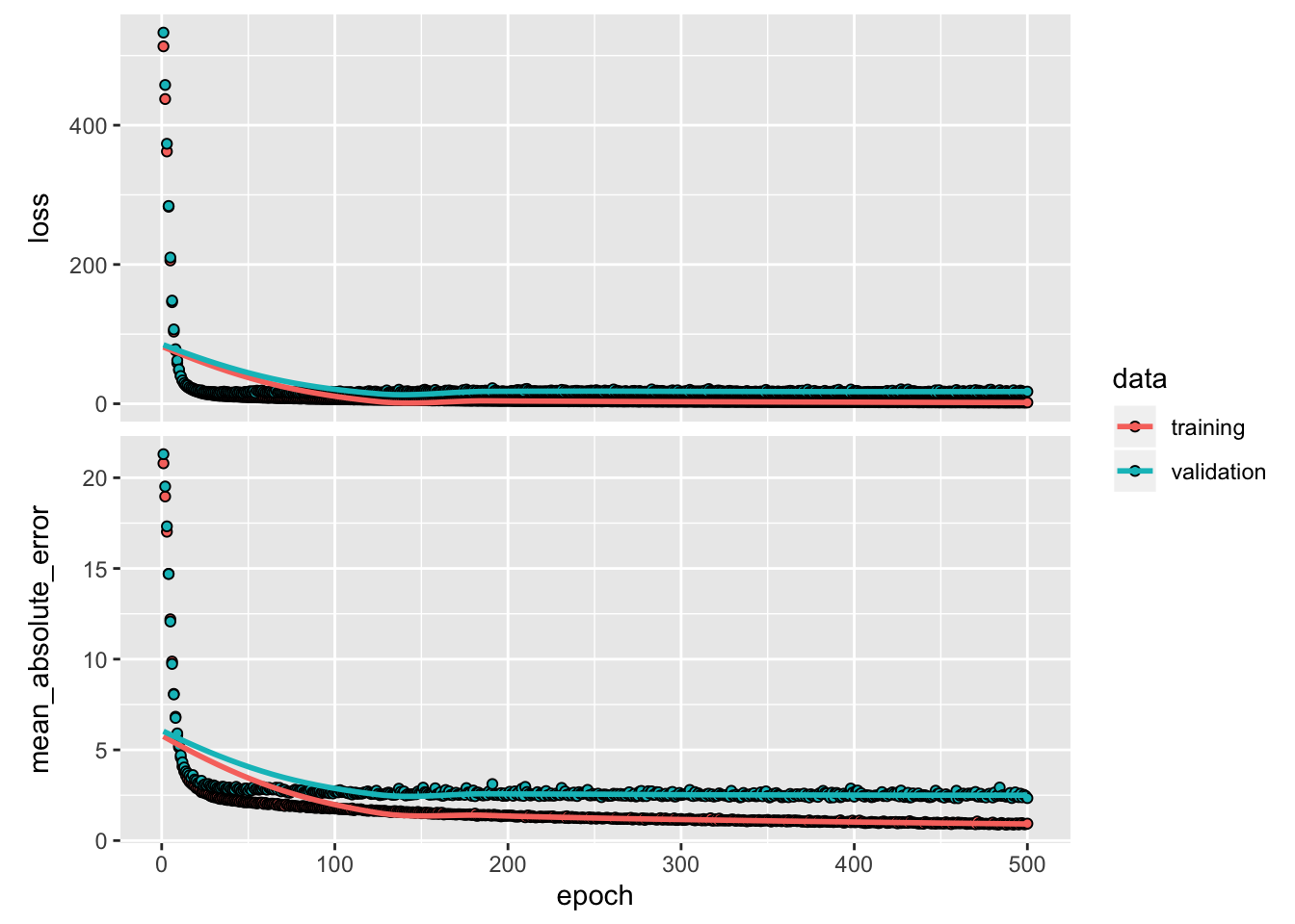

plot(history)

This graph shows little improvement in the model after about 200 epochs. Let’s update the fit method to automatically stop training when the validation score doesn’t improve. We’ll use a callback that tests a training condition for every epoch. If a set amount of epochs elapses without showing improvement, it automatically stops the training.

# The patience parameter is the amount of epochs to check for improvement.
early_stop <- callback_early_stopping(monitor = "val_loss", patience = 20)

model <- build_model()

history <- model %>% fit(
  x = train_df %>% select(-label),
  y = train_df$label,
  epochs = 500,
  validation_split = 0.2,
  verbose = 0,
  callbacks = list(early_stop)
)

plot(history)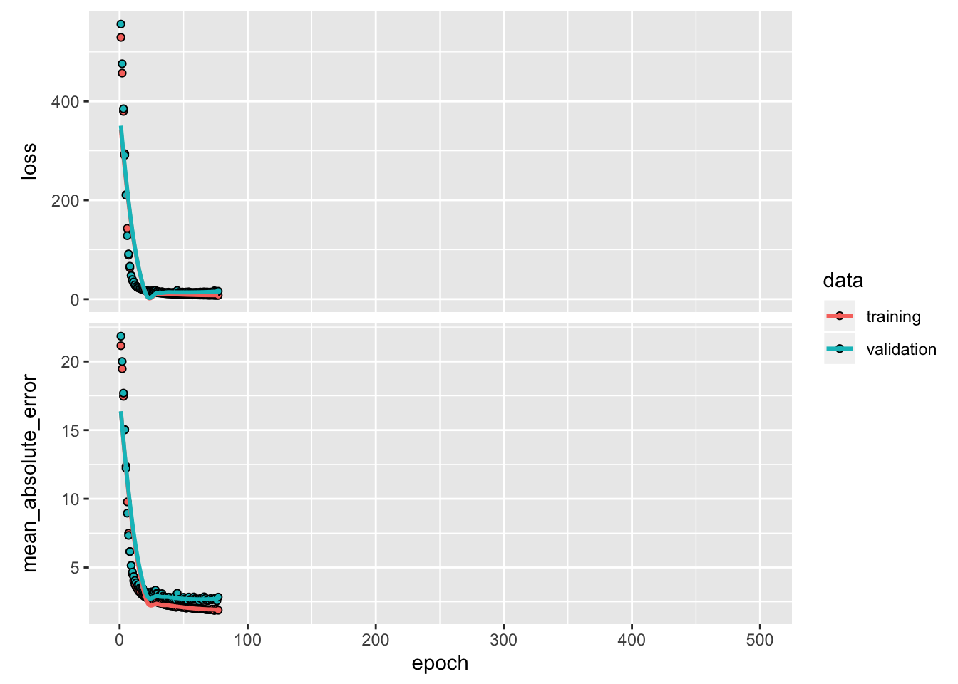

The graph shows the average error is about $2,500 dollars. Is this good? Well, $2,500 is not an insignificant amount when some of the labels are only $15,000.

Let’s see how did the model performs on the test set:

c(loss, mae) %<-% (model %>% evaluate(test_df %>% select(-label), test_df$label, verbose = 0))

paste0("Mean absolute error on test set: $", sprintf("%.2f", mae * 1000))

## [1] "Mean absolute error on test set: $3002.32"

Predict

Finally, predict some housing prices using data in the testing set:

test_predictions <- model %>% predict(test_df %>% select(-label))
test_predictions[ , 1]

##   [1]  7.759608 18.546511 21.525824 30.329552 26.206022 20.379061 28.972841
##   [8] 22.936476 19.548115 23.058081 18.773306 17.231783 16.081644 44.336926
##  [15] 19.217535 20.302008 28.332586 21.567612 20.574213 37.461048 11.579722
##  [22] 14.513885 21.496672 16.669203 22.553066 26.068880 30.536131 30.404364
##  [29] 10.445388 22.028477 19.943378 14.874774 33.198818 26.659334 17.360529
##  [36]  8.178129 15.533298 19.064489 19.243929 28.054504 31.655251 29.567472
##  [43] 14.953157 43.255310 31.586626 25.668932 28.000528 16.941755 24.727943
##  [50] 23.172396 36.855518 19.777802 12.556808 15.813701 36.187881 29.673326
##  [57] 13.030141 50.681965 33.722412 24.914156 25.301760 17.899117 14.868908
##  [64] 18.992828 24.683514 23.111195 13.744761 23.787327 14.203387  7.391667
##  [71] 37.876629 30.980328 26.656527 14.644408 27.063200 18.266968 21.141125
##  [78] 24.851347 36.980850 10.906940 20.344542 40.068722 15.938128 14.283166
##  [85] 18.121195 18.713694 21.409807 21.765066 22.943521 32.322598 19.994921
##  [92] 21.079947 26.719408 43.338303 36.935383 18.671057 37.789886 55.973999
##  [99] 27.252848 46.181122 32.272293 21.036985

Conclusion

This notebook introduced a few techniques to handle a regression problem.

Mean Squared Error (MSE) is a common loss function used for regression problems (different than classification problems).
Similarly, evaluation metrics used for regression differ from classification. A common regression metric is Mean Absolute Error (MAE).
When input data features have values with different ranges, each feature should be scaled independently.
If there is not much training data, prefer a small network with few hidden layers to avoid overfitting.
Early stopping is a useful technique to prevent overfitting.