Text Classification

Note: This tutorial requires TensorFlow version >= 2.1

This tutorial classifies movie reviews as positive or negative using the text of the review. This is an example of binary — or two-class — classification, an important and widely applicable kind of machine learning problem.

We’ll use the IMDB dataset that contains the text of 50,000 movie reviews from the Internet Movie Database. These are split into 25,000 reviews for training and 25,000 reviews for testing. The training and testing sets are balanced, meaning they contain an equal number of positive and negative reviews.

Let’s start and load Keras, as well as a few other required libraries.

library(keras)
library(dplyr)
library(ggplot2)
library(purrr)

Download the Movie Reviews dataset

We will use the Movie Reviews dataset created by Bo Pang and Lillian Lee. This dataset is redistributed with NLTK with permission from the authors.

The dataset can be found here and can be downloaded from the Kaggle UI or using the pins package.

If you are going to use pins follow this tutorial to register the Kaggle board. Then you can run:

paths <- pins::pin_get("nltkdata/movie-review", "kaggle")
# we only need the movie_review.csv file
path <- paths[1]

Now let’s read it to R using the read_csv funcntion from the readr package.

df <- readr::read_csv(path)

## Parsed with column specification:
## cols(
##   fold_id = col_double(),
##   cv_tag = col_character(),
##   html_id = col_double(),
##   sent_id = col_double(),
##   text = col_character(),
##   tag = col_character()
## )

head(df)

## # A tibble: 6 x 6
##   fold_id cv_tag html_id sent_id text                                 tag  
##     <dbl> <chr>    <dbl>   <dbl> <chr>                                <chr>
## 1       0 cv000    29590       0 films adapted from comic books have… pos  
## 2       0 cv000    29590       1 for starters , it was created by al… pos  
## 3       0 cv000    29590       2 to say moore and campbell thoroughl… pos  
## 4       0 cv000    29590       3 "the book ( or \" graphic novel , \… pos  
## 5       0 cv000    29590       4 in other words , don't dismiss this… pos  
## 6       0 cv000    29590       5 if you can get past the whole comic… pos

Explore the data

Let’s take a moment to understand the format of the data. The dataset has 60k rows, each one representing a movie review. The text column has the actual review and the tag represents shows us the classified sentiment for the review.

df %>% count(tag)

## # A tibble: 2 x 2
##   tag       n
##   <chr> <int>
## 1 neg   31783
## 2 pos   32937

Around half of the reviews are negative and the other half are positive. Here is an example of a review:

df$text[1]

## [1] "films adapted from comic books have had plenty of success , whether they're about superheroes ( batman , superman , spawn ) , or geared toward kids ( casper ) or the arthouse crowd ( ghost world ) , but there's never really been a comic book like from hell before ."

Let’s also split our dataset into training and testing:

training_id <- sample.int(nrow(df), size = nrow(df)*0.8)
training <- df[training_id,]
testing <- df[-training_id,]

It’s also useful to find out what is the distribution of the number of words in each review.

df$text %>% 
  strsplit(" ") %>% 
  sapply(length) %>% 
  summary()

##    Min. 1st Qu.  Median    Mean 3rd Qu.    Max. 
##    1.00   14.00   21.00   23.06   30.00  179.00

Prepare the data

The reviews — the text — must be converted to tensors before fed into the neural network. First, we create a dictionary and represent each of the 10,000 most common words by an integer. In this case, every review will be represented by a sequence of integers.

Then we can represent reviews in a couple of ways:

One-hot-encode the arrays to convert them into vectors of 0s and 1s. For example, the sequence [3, 5] would become a 10,000-dimensional vector that is all zeros except for indices 3 and 5, which are ones. Then, make this the first layer in our network — a dense layer — that can handle floating point vector data. This approach is memory intensive, though, requiring a num_words * num_reviews size matrix.
Alternatively, we can pad the arrays so they all have the same length, then create an integer tensor of shape num_examples * max_length. We can use an embedding layer capable of handling this shape as the first layer in our network.

In this tutorial, we will use the second approach. Now, let’s define our Text Vectorization layer, it will be responsible to take the string input and convert it to a Tensor.

num_words <- 10000
max_length <- 50
text_vectorization <- layer_text_vectorization(
  max_tokens = num_words, 
  output_sequence_length = max_length, 
)

Now, we need to adapt the Text Vectorization layer. It’s when we call adapt that the layer will learn about unique words in our dataset and assign an integer value for each one.

text_vectorization %>% 
  adapt(df$text)

We can now see the vocabulary is in our text vectorization layer.

# TODO see https://github.com/tensorflow/tensorflow/pull/34529
get_vocabulary(text_vectorization)

You can see how the text vectorization layer transforms it’s inputs:

text_vectorization(matrix(df$text[1], ncol = 1))

## tf.Tensor(
## [[  68 2835   30  359 1662   33   91 1056    5  632  631  321   41 7803
##    709 4865 1767   48 7600 1337  398 5161   48    2    1 1808 1800  148
##     17  140  109   90   69    3  359  408   40   30  503  142    0    0
##      0    0    0    0    0    0    0    0]], shape=(1, 50), dtype=int64)

Build the model

The neural network is created by stacking layers — this requires two main architectural decisions:

How many layers to use in the model?
How many hidden units to use for each layer?

In this example, the input data consists of an array of word-indices. The labels to predict are either 0 or 1. Let’s build a model for this problem:

input <- layer_input(shape = c(1), dtype = "string")

output <- input %>% 
  text_vectorization() %>% 
  layer_embedding(input_dim = num_words + 1, output_dim = 16) %>%
  layer_global_average_pooling_1d() %>%
  layer_dense(units = 16, activation = "relu") %>%
  layer_dropout(0.5) %>% 
  layer_dense(units = 1, activation = "sigmoid")

model <- keras_model(input, output)

The layers are stacked sequentially to build the classifier:

The first layer is an embedding layer. This layer takes the integer-encoded vocabulary and looks up the embedding vector for each word-index. These vectors are learned as the model trains. The vectors add a dimension to the output array. The resulting dimensions are: (batch, sequence, embedding).
Next, a global_average_pooling_1d layer returns a fixed-length output vector for each example by averaging over the sequence dimension. This allows the model to handle input of variable length, in the simplest way possible.
This fixed-length output vector is piped through a fully-connected (dense) layer with 16 hidden units.
The last layer is densely connected with a single output node. Using the sigmoid activation function, this value is a float between 0 and 1, representing a probability, or confidence level.

Hidden units

The above model has two intermediate or “hidden” layers, between the input and output. The number of outputs (units, nodes, or neurons) is the dimension of the representational space for the layer. In other words, the amount of freedom the network is allowed when learning an internal representation.

If a model has more hidden units (a higher-dimensional representation space), and/or more layers, then the network can learn more complex representations. However, it makes the network more computationally expensive and may lead to learning unwanted patterns — patterns that improve performance on training data but not on the test data. This is called overfitting, and we’ll explore it later.

Loss function and optimizer

A model needs a loss function and an optimizer for training. Since this is a binary classification problem and the model outputs a probability (a single-unit layer with a sigmoid activation), we’ll use the binary_crossentropy loss function.

This isn’t the only choice for a loss function, you could, for instance, choose mean_squared_error. But, generally, binary_crossentropy is better for dealing with probabilities — it measures the “distance” between probability distributions, or in our case, between the ground-truth distribution and the predictions.

Later, when we are exploring regression problems (say, to predict the price of a house), we will see how to use another loss function called mean squared error.

Now, configure the model to use an optimizer and a loss function:

model %>% compile(
  optimizer = 'adam',
  loss = 'binary_crossentropy',
  metrics = list('accuracy')
)

Train the model

Train the model for 20 epochs in mini-batches of 512 samples. This is 20 iterations over all samples in the x_train and y_train tensors. While training, monitor the model’s loss and accuracy on the 10,000 samples from the validation set:

history <- model %>% fit(
  training$text,
  as.numeric(training$tag == "pos"),
  epochs = 10,
  batch_size = 512,
  validation_split = 0.2,
  verbose=2
)

## Train on 41420 samples, validate on 10356 samples
## Epoch 1/10
## 41420/41420 - 1s - loss: 0.6921 - accuracy: 0.5185 - val_loss: 0.6898 - val_accuracy: 0.5410
## Epoch 2/10
## 41420/41420 - 0s - loss: 0.6862 - accuracy: 0.5600 - val_loss: 0.6805 - val_accuracy: 0.5965
## Epoch 3/10
## 41420/41420 - 0s - loss: 0.6716 - accuracy: 0.6050 - val_loss: 0.6633 - val_accuracy: 0.6400
## Epoch 4/10
## 41420/41420 - 0s - loss: 0.6468 - accuracy: 0.6515 - val_loss: 0.6399 - val_accuracy: 0.6619
## Epoch 5/10
## 41420/41420 - 0s - loss: 0.6161 - accuracy: 0.6796 - val_loss: 0.6184 - val_accuracy: 0.6747
## Epoch 6/10
## 41420/41420 - 0s - loss: 0.5875 - accuracy: 0.7029 - val_loss: 0.6039 - val_accuracy: 0.6808
## Epoch 7/10
## 41420/41420 - 1s - loss: 0.5632 - accuracy: 0.7212 - val_loss: 0.5963 - val_accuracy: 0.6831
## Epoch 8/10
## 41420/41420 - 0s - loss: 0.5448 - accuracy: 0.7336 - val_loss: 0.5917 - val_accuracy: 0.6863
## Epoch 9/10
## 41420/41420 - 0s - loss: 0.5297 - accuracy: 0.7442 - val_loss: 0.5937 - val_accuracy: 0.6842
## Epoch 10/10
## 41420/41420 - 0s - loss: 0.5165 - accuracy: 0.7539 - val_loss: 0.5953 - val_accuracy: 0.6868

Evaluate the model

And let’s see how the model performs. Two values will be returned. Loss (a number which represents our error, lower values are better), and accuracy.

results <- model %>% evaluate(testing$text, as.numeric(testing$tag == "pos"), verbose = 0)
results

## $loss
## [1] 0.5940198
## 
## $accuracy
## [1] 0.6830192

This fairly naive approach achieves an accuracy of about 68%. With more advanced approaches, the model should get closer to 85%.

Create a graph of accuracy and loss over time

fit returns a keras_training_history object whose metrics slot contains loss and metrics values recorded during training. You can conveniently plot the loss and metrics curves like so:

plot(history)

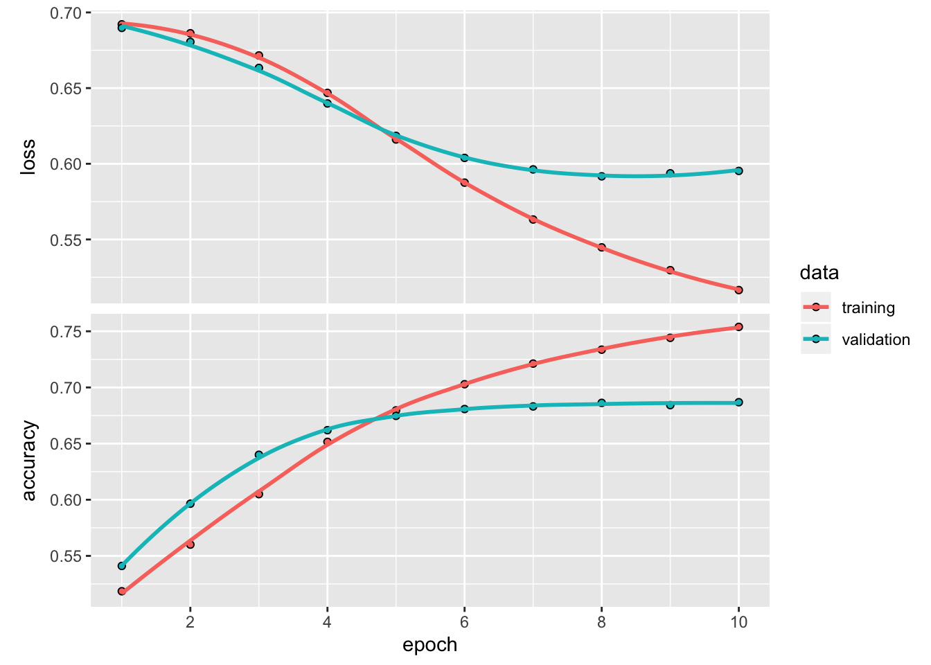
The evolution of loss and metrics can also be seen during training in the RStudio Viewer pane.

Notice the training loss decreases with each epoch and the training accuracy increases with each epoch. This is expected when using gradient descent optimization — it should minimize the desired quantity on every iteration.